Difference between revisions of "Local fields"
| (43 intermediate revisions by 4 users not shown) | |||
| Line 1: | Line 1: | ||
In this | In this module you will learn how to calculate the macroscopic dielectric function in 2D hBN. | ||
[[File:Yambo-CH7.png|none| | == Background == | ||
The microscopic dielectric function is related to X by: | [[File:Yambo-handbook-v4.1.2-p-4.png|thumb|Cheatsheet on LFE|150px]] | ||
The macroscopic dielectric function is obtained by including the so-called local field effects (LFE) in the calculation of the response function. Within the time-dependent DFT formalism this is achieved by solving the Dyson equation for the susceptibility ''X''. In reciprocal space this is given by: | |||
[[File:Yambo-CH7.png|none|x50px|Yambo tutorial image]] | |||
The microscopic dielectric function is related to ''X'' by: | |||
[[File:Yambo-CH5.png|none|x30px|Yambo tutorial image]] | [[File:Yambo-CH5.png|none|x30px|Yambo tutorial image]] | ||
and the macroscopic dielectric function is obtained by taking the (0,0) component of the inverse microscopic one: | and the macroscopic dielectric function is obtained by taking the (0,0) component of the inverse microscopic one: | ||
[[File:Yambo-CH6.png|none|x60px|Yambo tutorial image]] | [[File:Yambo-CH6.png|none|x60px|Yambo tutorial image]] | ||
Experimental observables like the optical absorption and the electron energy loss can be obtained from the macroscopic dielectric function: | |||
[[File:Yambo-CH8.png|none|x60px|Yambo tutorial image]] | |||
In the following we will neglect the ''f <sup> xc</sup>'' term: we perform the calculation at the RPA level and consider just the Hartree term (from ''v<sub>G</sub>'') in the kernel. If we also neglect the Hartree term, we arrive back at the independent particle approximation, since there is no kernel and ''X = X<sub>0</sub>''. | |||
== Prerequisites == | == Prerequisites == | ||
* You must first complete the | * You must first complete the [[Tutorials#How to use Yambo|How to use Yambo]] modules | ||
'''You will need''': | '''You will need''': | ||
* The <code>SAVE</code> databases for 2D hBN | * The <code>SAVE</code> databases for 2D hBN | ||
* The <code>yambo</code> executable | * The <code>yambo</code> executable | ||
* <code>gnuplot</code> | * <code>gnuplot</code> for plotting spectra | ||
== Choosing input parameters == | == Choosing input parameters == | ||
Enter the folder for 2D hBN that contains the SAVE directory, and generate the input file. From <code>yambo - | Enter the folder for 2D hBN that contains the SAVE directory, and generate the input file. From <code>yambo -h</code> you should understand that the correct option is <code>yambo -optics c -kernel hartree</code> (or <code>yambo -o c -k hartree</code>). Let's start by running the calculation for light polarization ''q'' in the plane of the BN sheet: | ||
$ cd YAMBO_TUTORIALS/hBN-2D/YAMBO | $ cd YAMBO_TUTORIALS/hBN-2D/YAMBO | ||
$ yambo ''(Initialization)'' | |||
$ yambo -F yambo.in_RPA -V RL -J q100 -o c -k hartree | $ yambo -F yambo.in_RPA -V RL -J q100 -o c -k hartree | ||
and | We thus use a new input file ''yambo.in_RPA'', switch on the <code>FFTGvecs</code> variable, and label all outputs/databases with a ''q100'' tag. Make sure to set/modify all of the following variables to: | ||
FFTGvecs= '''6 Ry''' # [FFT] Plane-waves | [[Variables#FFTGvecs|FFTGvecs]]= '''6 Ry''' # [FFT] Plane-waves | ||
Chimod= "Hartree" # [X] IP/Hartree/ALDA/LRC/BSfxc | [[Variables#Chimod|Chimod]]= "Hartree" # [X] IP/Hartree/ALDA/LRC/BSfxc | ||
NGsBlkXd= '''3 | [[Variables#NGsBlkXd|NGsBlkXd]]= ''' 3 Ry''' # [Xd] Response block size | ||
% QpntsRXd | % [[Variables#QpntsRXd|QpntsRXd]] | ||
1 | 1 | # [Xd] Transferred momenta | 1 | 1 | # [Xd] Transferred momenta | ||
% | % | ||
% EnRngeXd | % [[Variables#EnRngeXd|EnRngeXd]] | ||
0.00000 | 20.00000 | eV # [Xd] Energy range | 0.00000 | 20.00000 | eV # [Xd] Energy range | ||
% | % | ||
% DmRngeXd | % [[Variables#DmRngeXd|DmRngeXd]] | ||
0.200000 | 0.200000 | eV # [Xd] Damping range | 0.200000 | 0.200000 | eV # [Xd] Damping range | ||
% | % | ||
ETStpsXd= 2001 # [Xd] Total Energy steps | [[Variables#ETStpsXd|ETStpsXd]]= 2001 # [Xd] Total Energy steps | ||
% LongDrXd | % [[Variables#LongDrXd|LongDrXd]] | ||
1.000000 | 0.000000 | 0.000000 | # [Xd] [cc] Electric Field | 1.000000 | 0.000000 | 0.000000 | # [Xd] [cc] Electric Field | ||
% | % | ||
In this input file, we have | In this input file, we have: | ||
* | * We evaluate the q-->0 response function choosing the direction for the limit parallel in the plane of the hBN sheet | ||
* A wider energy range than before, and more broadening | * A wider energy range than before, and more broadening | ||
* Selected the Hartree kernel, and | * Selected the Hartree kernel, and expanded G-vectors in the screening up to 3 Ry (about 85 G-vectors) | ||
$ yambo -F yambo.in_RPA | ==LFEs in periodic direction== | ||
and let's compare the absorption with and without the local fields included. By inspecting the 'o-q100.eps_q1_inv_rpa_dyson' file | Now let's run the code with this new input file (CECAM in serial: about 2mins; parallel 4 tasks: 50s) | ||
$ yambo -F yambo.in_RPA -J q100 | |||
and let's compare the absorption with and without the local fields included. By inspecting the ''o-q100.eps_q1_inv_rpa_dyson'' file we find | |||
that this information is given in the 2nd and 4th columns, respectively: | |||
$ head -n30 o-q100.eps_q1_inv_rpa_dyson | |||
# Absorption @ Q(1) [q->0 direction] : 1.0000000 0.0000000 0.0000000 | |||
# E/ev[1] EPS-Im[2] EPS-Re[3] EPSo-Im[4] EPSo-Re[5] | # E/ev[1] EPS-Im[2] EPS-Re[3] EPSo-Im[4] EPSo-Re[5] | ||
Plot the result: | |||
$ gnuplot | $ gnuplot | ||
gnuplot > plot "o-q100.eps_q1_inv_rpa_dyson" u 1:2 t " | gnuplot> plot "o-q100.eps_q1_inv_rpa_dyson" u 1:2 w l t "RPA-LFA","o-q100.eps_q1_inv_rpa_dyson" u 1:4 w l t "noLFE", "o-q100.eel_q1_inv_rpa_dyson" u 1:4 w l ls 7 dt 2 t "EELS" | ||
[[File:CH-LFE4.png|none|600px|Yambo tutorial image]] | [[File:CH-LFE4.png|none|600px|Yambo tutorial image]] | ||
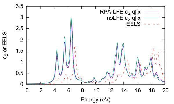
It is clear that there is little influence of local fields in this case. We have also | It is clear that there is little influence of local fields in this case. This is generally the case for semiconductors or materials with a smoothly varying electronic density. We have also shown the EELS spectrum (''o-q100.eel_q1_inv_rpa_dyson'') for comparison. | ||
==LFEs in non-periodic direction== | |||
Now let's switch to ''q'' perpendicular to the BN plane: | Now let's switch to ''q'' perpendicular to the BN plane: | ||
$ yambo -F yambo.in_RPA -V RL | $ yambo -F yambo.in_RPA -V RL -o c -k hartree ''and set'' | ||
... | ... | ||
% LongDrXd | % [[Variables#LongDrXd|LongDrXd]] | ||
0.000000 | 0.000000 | ''1.000000'' | # [Xd] [cc] Electric Field | 0.000000 | 0.000000 | '''1.000000''' | # [Xd] [cc] Electric Field | ||
% | % | ||
. | |||
$ yambo -F yambo.in_RPA -V RL -J ''q001'' | You can try out the default parallel usage now, or run again in serial, i.e. | ||
$ yambo -F yambo.in_RPA -V RL -J '''q001''' ''(serial)'' | |||
$ mpirun -np 4 yambo -F yambo.in_RPA -J '''q001''' & ''(parallel, MPI only, 4 tasks)'' | |||
As noted previously, the ''log'' files in parallel appear in the LOG folder, you can follow the execution with <code>tail -F LOG/l-q001_optics_chi_CPU_1</code> . | |||
Plotting the output file: | Plotting the output file: | ||
$ gnuplot | $ gnuplot | ||
gnuplot> plot "o-q001.eps_q1_inv_rpa_dyson" u 1:2 | gnuplot> plot "o-q001.eps_q1_inv_rpa_dyson" u 1:2 w l,"o-q001.eps_q1_inv_rpa_dyson" u 1:4 w l | ||
[[File:CH- | [[File:CH-LFE6.png|none|600px|Yambo tutorial image]] | ||
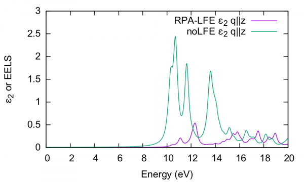
In this case, the absorption is strongly | In this case, the absorption is strongly blueshifted with respect to the in-plane absorption. Furthermore, the influence of local fields is striking, and quenches the spectrum strongly. This is the well known depolarization effect. Local field effects are much stronger in the perpendicular direction because the charge inhomogeneity is dramatic. Many G-vectors are needed to account for the sharp change in the potential across the BN-vacuum interface. | ||
In order to understand this, we plot the electron energy loss spectrum for this component and compare with the absorption: | ==Absorption versus EELS== | ||
In order to understand this further, we plot the electron energy loss spectrum for this component and compare with the absorption: | |||
$ gnuplot | $ gnuplot | ||
gnuplot > plot "o-q001.eps_q1_inv_rpa_dyson | gnuplot > plot "o-q001.eps_q1_inv_rpa_dyson" w l,"o-q001.eel_q1_inv_rpa_dyson" w l | ||
[[File:CH-LFE5.png|none|600px|Yambo tutorial image]] | [[File:CH-LFE5.png|none|600px|Yambo tutorial image]] | ||
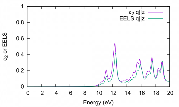
The conclusion is that the | The conclusion is that the absorption and EELS coincide for isolated systems. | ||
<!--You should verify that this is not the case for the periodic (in-plane) direction. This is not true, for large cell it also end up to give the same Abs/EELS--> | |||
To understand why this is, you need to consider the role of the ''macroscopic'' screening in the response function and the long-range part of the Coulomb potential. | |||
See e.g.<ref>TDDFT from molecules to solids: The role of long‐range interactions, F. Sottile et al, International journal of quantum chemistry 102 (5), 684-701 (2005)</ref> | |||
==Summary== | |||
From this tutorial you've learned: | From this tutorial you've learned: | ||
* How to compute | * How to compute the macroscopic dielectric function by solving the Dyson equation for ''X'' in G-space | ||
* The connection between absorption and EELS in low-dimensional systems | |||
* | |||
== | <br> | ||
{| style="width:100%" border="1" | |||
|style="width:15%; text-align:left"|Prev: Back to [[First_steps:_a_walk_through_from_DFT_to_optical_properties|First steps]] | |||
|style="width:70%; text-align:center"|Now: [[Tutorials|Tutorials Home]] --> [[First_steps:_a_walk_through_from_DFT_to_optical_properties|First steps]] --> [[2D_material:_h-BN_sheet|2D hBN]] --> [[Local_fields|RPA with Local Fields]] | |||
|style="width:15%; text-align:right"|Next: Back to [[First_steps:_a_walk_through_from_DFT_to_optical_properties|First steps]] | |||
|- | |||
|} | |||
Latest revision as of 09:08, 30 March 2021
In this module you will learn how to calculate the macroscopic dielectric function in 2D hBN.
Background
The macroscopic dielectric function is obtained by including the so-called local field effects (LFE) in the calculation of the response function. Within the time-dependent DFT formalism this is achieved by solving the Dyson equation for the susceptibility X. In reciprocal space this is given by:
The microscopic dielectric function is related to X by:
and the macroscopic dielectric function is obtained by taking the (0,0) component of the inverse microscopic one:
Experimental observables like the optical absorption and the electron energy loss can be obtained from the macroscopic dielectric function:
In the following we will neglect the f xc term: we perform the calculation at the RPA level and consider just the Hartree term (from vG) in the kernel. If we also neglect the Hartree term, we arrive back at the independent particle approximation, since there is no kernel and X = X0.
Prerequisites
- You must first complete the How to use Yambo modules
You will need:
- The
SAVEdatabases for 2D hBN - The
yamboexecutable gnuplotfor plotting spectra
Choosing input parameters
Enter the folder for 2D hBN that contains the SAVE directory, and generate the input file. From yambo -h you should understand that the correct option is yambo -optics c -kernel hartree (or yambo -o c -k hartree). Let's start by running the calculation for light polarization q in the plane of the BN sheet:
$ cd YAMBO_TUTORIALS/hBN-2D/YAMBO
$ yambo        (Initialization)
$ yambo -F yambo.in_RPA -V RL -J q100 -o c -k hartree
We thus use a new input file yambo.in_RPA, switch on the FFTGvecs variable, and label all outputs/databases with a q100 tag. Make sure to set/modify all of the following variables to:
FFTGvecs=     6        Ry    # [FFT] Plane-waves
Chimod= "Hartree"            # [X] IP/Hartree/ALDA/LRC/BSfxc
NGsBlkXd=     3        Ry    # [Xd] Response block size
% QpntsRXd
 1 |  1 |                   # [Xd] Transferred momenta
%
% EnRngeXd
 0.00000 | 20.00000 | eV    # [Xd] Energy range
%
% DmRngeXd
0.200000 | 0.200000 | eV    # [Xd] Damping range
%
ETStpsXd= 2001               # [Xd] Total Energy steps
% LongDrXd
1.000000 | 0.000000 | 0.000000 |        # [Xd] [cc] Electric Field
%
In this input file, we have:
- We evaluate the q-->0 response function choosing the direction for the limit parallel in the plane of the hBN sheet
- A wider energy range than before, and more broadening
- Selected the Hartree kernel, and expanded G-vectors in the screening up to 3 Ry (about 85 G-vectors)
LFEs in periodic direction
Now let's run the code with this new input file (CECAM in serial: about 2mins; parallel 4 tasks: 50s)
$ yambo -F yambo.in_RPA -J q100
and let's compare the absorption with and without the local fields included. By inspecting the o-q100.eps_q1_inv_rpa_dyson file we find that this information is given in the 2nd and 4th columns, respectively:
$ head -n30 o-q100.eps_q1_inv_rpa_dyson
# Absorption @ Q(1) [q->0 direction] : 1.0000000  0.0000000  0.0000000
#  E/ev[1]     EPS-Im[2]   EPS-Re[3]   EPSo-Im[4]  EPSo-Re[5]
Plot the result:
$ gnuplot
gnuplot> plot "o-q100.eps_q1_inv_rpa_dyson" u 1:2 w l t "RPA-LFA","o-q100.eps_q1_inv_rpa_dyson" u 1:4 w l t "noLFE", "o-q100.eel_q1_inv_rpa_dyson" u 1:4 w l ls 7 dt 2 t "EELS"
It is clear that there is little influence of local fields in this case. This is generally the case for semiconductors or materials with a smoothly varying electronic density. We have also shown the EELS spectrum (o-q100.eel_q1_inv_rpa_dyson) for comparison.
LFEs in non-periodic direction
Now let's switch to q perpendicular to the BN plane:
$ yambo -F yambo.in_RPA -V RL -o c -k hartree        and set
...
% LongDrXd
0.000000 | 0.000000 | 1.000000 |        # [Xd] [cc] Electric Field
%
You can try out the default parallel usage now, or run again in serial, i.e.
$ yambo -F yambo.in_RPA -V RL -J q001       (serial)
$ mpirun -np 4 yambo -F yambo.in_RPA -J q001 &      (parallel, MPI only, 4 tasks)
As noted previously, the log files in parallel appear in the LOG folder, you can follow the execution with tail -F LOG/l-q001_optics_chi_CPU_1 .
Plotting the output file:
$ gnuplot
gnuplot> plot "o-q001.eps_q1_inv_rpa_dyson" u 1:2 w l,"o-q001.eps_q1_inv_rpa_dyson" u 1:4 w l
In this case, the absorption is strongly blueshifted with respect to the in-plane absorption. Furthermore, the influence of local fields is striking, and quenches the spectrum strongly. This is the well known depolarization effect. Local field effects are much stronger in the perpendicular direction because the charge inhomogeneity is dramatic. Many G-vectors are needed to account for the sharp change in the potential across the BN-vacuum interface.
Absorption versus EELS
In order to understand this further, we plot the electron energy loss spectrum for this component and compare with the absorption:
$ gnuplot
gnuplot > plot "o-q001.eps_q1_inv_rpa_dyson" w l,"o-q001.eel_q1_inv_rpa_dyson" w l
The conclusion is that the absorption and EELS coincide for isolated systems. To understand why this is, you need to consider the role of the macroscopic screening in the response function and the long-range part of the Coulomb potential. See e.g.[1]
Summary
From this tutorial you've learned:
- How to compute the macroscopic dielectric function by solving the Dyson equation for X in G-space
- The connection between absorption and EELS in low-dimensional systems
| Prev: Back to First steps | Now: Tutorials Home --> First steps --> 2D hBN --> RPA with Local Fields | Next: Back to First steps |
- ↑ TDDFT from molecules to solids: The role of long‐range interactions, F. Sottile et al, International journal of quantum chemistry 102 (5), 684-701 (2005)


