Difference between revisions of "Correlation effects in the non-linear response"
| (29 intermediate revisions by 2 users not shown) | |||
| Line 4: | Line 4: | ||
==Background== | ==Background== | ||
In real-time simulations using TDSE, correlation effects are determined by the choice of the Hamiltonian | In real-time simulations using TDSE, correlation effects are determined by the choice of the Hamiltonian <math> H^{\text{sys}}_{\mathbf k} </math> that enters in the equations of motion(EOM). | ||
Yambo can use different models for the system Hamiltonian: | Yambo can use different models for the system Hamiltonian: | ||
| Line 17: | Line 17: | ||
<math> H^{\text{QP}}_{\mathbf k} \equiv H^{\text{KS}}_{\mathbf k} + \Delta H_{\mathbf k}. </math> | <math> H^{\text{QP}}_{\mathbf k} \equiv H^{\text{KS}}_{\mathbf k} + \Delta H_{\mathbf k}. </math> | ||
where <math> \Delta H_{\mathbf k} </math> is the GW correction or scissor operator, estimated from the Many-Body Perturbation Theory (Ref. <ref name=" | where <math> \Delta H_{\mathbf k} </math> is the GW correction or scissor operator, estimated from the Many-Body Perturbation Theory (Ref. <ref name="Aryasetiawan1998"/>), and then applied to the KS eigenvalues. | ||
* The RPA model (or Time-dependent Hartree), | * The RPA model (or Time-dependent Hartree), | ||
| Line 31: | Line 31: | ||
The term <math> V_{xc}(\mathbf r)[\Delta\rho] </math> is the time-dependent exchange-correlation potential. | The term <math> V_{xc}(\mathbf r)[\Delta\rho] </math> is the time-dependent exchange-correlation potential. | ||
* The Time Dependent-Density Polarization Function Theory (TD-DPFT) model, at present different functionals are implemented in Yambo, for more details see Ref. <ref name=" | * The Time Dependent-Density Polarization Function Theory (TD-DPFT) model, at present different functionals are implemented in Yambo, for more details see Ref. <ref name="Gruning2016"/>: | ||
<math> H^{\text{TD-DFTP}}_{\mathbf k} \equiv H^{\text{KS}}_{\mathbf k} + V_h(\mathbf r)[\Delta\rho] + V_{xc}(\mathbf r)[\Delta\rho] -\Omega \mathcal{E}^s(t) \cdot \nabla_{\mathbf k} </math> | <math> H^{\text{TD-DFTP}}_{\mathbf k} \equiv H^{\text{KS}}_{\mathbf k} + V_h(\mathbf r)[\Delta\rho] + V_{xc}(\mathbf r)[\Delta\rho] -\Omega \mathcal{E}^s(t) \cdot \nabla_{\mathbf k} </math> | ||
where <math> \mathcal{E}^s(t) </math> is the Kohn-Sham macroscopic field (see Ref. <ref name=" | where <math> \mathcal{E}^s(t) </math> is the Kohn-Sham macroscopic field (see Ref. <ref name="Gruning2016"/>, <ref name="Martin1997"/>). | ||
==Prerequisites== | ==Prerequisites== | ||
| Line 149: | Line 149: | ||
% | % | ||
The | The <math> \alpha </math> parameter for AlAs has been taken from Ref. <ref name="Botti"/>. The results is: | ||
[[File:AlAs LRC results.png|600px|center| SHG in AlAs at TD-DFTP level with LRC kernel]] | [[File:AlAs LRC results.png|600px|center| SHG in AlAs at TD-DFTP level with LRC kernel]] | ||
Plot data are available [http://www.attaccalite.com/lumen/tutorials/AlAs/AlAs_TDDFT_results.tgz here]. | Plot data are available [http://www.attaccalite.com/lumen/tutorials/AlAs/AlAs_TDDFT_results.tgz here]. | ||
Notice that different models for the \( \alpha \) parameter have been proposed in the literature, see Ref. <ref name=" | Notice that different models for the \( \alpha \) parameter have been proposed in the literature, see Ref. <ref name="Gruning2016"/> for a discussion. | ||
Finally, in Yambo we implemented also the Jelium-with gap model NLCorrelation="JGM" that provides an automatic estimation of the \( \alpha \) parameters for each material, see Ref. <ref name=" | Finally, in Yambo we implemented also the Jelium-with gap model NLCorrelation="JGM" that provides an automatic estimation of the \( \alpha \) parameters for each material, see Ref. <ref name="Gruning2016"/> for a discussion on this approximation. | ||
==SHG at the TD-BSE level== | ==SHG at the TD-BSE level== | ||
Second-harmonic generation can be calculated also the TD-BSE level, the procedure is the same of the [[Real_time_Bethe-Salpeter_Equation_(TDSE) | linear response case]]: the first one has to calculate the collisions integrals (see appendix of Ref.<ref | Second-harmonic generation can be calculated also the TD-BSE level, the procedure is the same of the [[Real_time_Bethe-Salpeter_Equation_(TDSE) | linear response case]]: the first one has to calculate the collisions integrals (see appendix of Ref.<ref name="Attaccalite2011"/>) and then can run simulation for the non-linear response as it is shown in this tutorial. | ||
Hereafter we will briefly repeat the steps necessary to obtain SHG including excitonic effects. | |||
1) Download DFT wave-functions and input file here: [http://media.yambo-code.eu/educational/tutorials/files/hBN-2D-RT.tar.gz hBN-2D-RT.tar.gz] <br> | |||
2) Run the setup <br> | |||
3) Remove symmetries<br> | |||
use the command <span style="color:blue">ypp_nl -y</span> | |||
fixsyms | |||
# [R] Remove symmetries not consistent with an external perturbation | |||
% Efield1 | |||
<span style="color:red"> 0.000000 | 1.000000 | 0.000000 | </span> # First external Electric Field | |||
% | |||
% Efield2 | |||
0.000000 | 0.000000 | 0.000000 | # Additional external Electric Field | |||
% | |||
BField= 0.000000 T # [MAG] Magnetic field modulus | |||
Bpsi= 0.000000 deg # [MAG] Magnetic field psi angle [degree] | |||
Btheta= 0.000000 deg # [MAG] Magnetic field theta angle [degree] | |||
<span style="color:red">RmTimeRev </span> # Remove Time Reversal | |||
then go in the <span style="color:blue">FixSymm </span>folder and run the setup again | |||
4) Generate collisions integrals | |||
generate collision for HSEX using the command: <span style="color:blue">yambo_nl -X s -e -v h+sex</span> | |||
em1s # [R][Xs] Statically Screened Interaction | |||
collisions # [R] Collisions | |||
dipoles # [R] Oscillator strenghts (or dipoles) | |||
DIP_Threads=0 # [OPENMP/X] Number of threads for dipoles | |||
X_Threads=0 # [OPENMP/X] Number of threads for response functions | |||
RT_Threads=0 # [OPENMP/RT] Number of threads for real-time | |||
Chimod= "HARTREE" # [X] IP/Hartree/ALDA/LRC/PF/BSfxc | |||
% BndsRnXs | |||
1 | 20 | # [Xs] Polarization function bands | |||
% | |||
<span style="color:red"> NGsBlkXs= 3000 mHa </span> # [Xs] Response block size | |||
% LongDrXs | |||
1.000000 | 0.000000 | 0.000000 | # [Xs] [cc] Electric Field | |||
% | |||
% COLLBands | |||
<span style="color:red"> 4 | 5 | </span> # [COLL] Bands for the collisions | |||
% | |||
HXC_Potential= "SEX+HARTREE" # [SC] SC HXC Potential | |||
<span style="color:red">HARRLvcs= 1000 mHa</span> # [HA] Hartree RL components | |||
<span style="color:red">EXXRLvcs= 1000 mHa</span> # [XX] Exchange RL components | |||
<span style="color:red">CORRLvcs= 1000 mHa</span> # [GW] Correlation RL components | |||
5) Run the SHG calculation including collisions, with the command: <span style="color:blue">yambo_nl -u n -V qp</span> | |||
nloptics # [R] Non-linear spectroscopy | |||
DIP_Threads=0 # [OPENMP/X] Number of threads for dipoles | |||
NL_Threads=0 # [OPENMP/NL] Number of threads for nl-optics | |||
% NLBands | |||
<span style="color:red"> 4 | 5 | </span> # [NL] Bands range | |||
% | |||
NLverbosity= "high" # [NL] Verbosity level (low | high) | |||
<span style="color:red">NLtime=42.000000</span> fs # [NL] Simulation Time | |||
<span style="color:red">NLintegrator= "CRANKNIC" </span> # [NL] Integrator ("EULEREXP/RK2/RK4/RK2EXP/HEUN/INVINT/CRANKNIC") | |||
<span style="color:red">NLCorrelation= "SEX" </span> # [NL] Correlation ("IPA/HARTREE/TDDFT/LRC/LRW/JGM/SEX") | |||
NLLrcAlpha= 0.000000 # [NL] Long Range Correction | |||
% NLEnRange | |||
<span style="color:red"> 2.000000 | 8.000000 | </span> eV # [NL] Energy range | |||
% | |||
NLEnSteps= 80 # [NL] Energy steps | |||
NLDamping= 0.200000 eV # [NL] Damping (or dephasing) | |||
RADLifeTime=-1.000000 fs # [RT] Radiative life-time (if negative Yambo sets it equal to Phase_LifeTime in NL) | |||
#EvalCurrent # [NL] Evaluate the current | |||
#FrPolPerdic # [DIP] Force periodicity of polarization respect to the external field | |||
<span style="color:red">HARRLvcs= 1000 mHa </span> # [HA] Hartree RL components | |||
<span style="color:red">EXXRLvcs= 1000 mHa </span> # [XX] Exchange RL components | |||
GfnQPdb= "none" # [EXTQP G] Database action | |||
GfnQP_INTERP_NN= 1 # [EXTQP G] Interpolation neighbours (NN mode) | |||
GfnQP_INTERP_shells= 20.00000 # [EXTQP G] Interpolation shells (BOLTZ mode) | |||
GfnQP_DbGd_INTERP_mode= "NN" # [EXTQP G] Interpolation DbGd mode | |||
% GfnQP_E | |||
<span style="color:red"> 3.000000 | 1.000000 | 1.000000 | </span> # [EXTQP G] E parameters (c/v) eV|adim|adim | |||
% | |||
............. | |||
% Field1_Freq | |||
0.100000 | 0.100000 | eV # [RT Field1] Frequency | |||
% | |||
Field1_NFreqs= 1 # [RT Field1] Frequency | |||
Field1_Int= 1000.00 kWLm2 # [RT Field1] Intensity | |||
Field1_Width= 0.000000 fs # [RT Field1] Width | |||
Field1_kind= "SOFTSIN" # [RT Field1] Kind(SIN|COS|RES|ANTIRES|GAUSS|DELTA|QSSIN) | |||
Field1_pol= "linear" # [RT Field1] Pol(linear|circular) | |||
% Field1_Dir | |||
<span style="color:red"> 0.000000 | 1.000000 | 0.000000 | </span> # [RT Field1] Versor | |||
% | |||
6) Use the command <span style="color:blue">ypp_nl -u </span> to analyze the result | |||
nonlinear # [R] Non-linear response analysis | |||
<span style="color:red">Xorder= 4 </span> # Max order of the response/exc functions | |||
% TimeRange | |||
<span style="color:red">40.000 | -1.00000 | </span> fs # Time-window where processing is done | |||
% | |||
ETStpsRt= 200 # Total Energy steps | |||
% EnRngeRt | |||
0.00000 | 20.00000 | eV # Energy range | |||
% | |||
DampMode= "NONE" # Damping type ( NONE | LORENTZIAN | GAUSSIAN ) | |||
DampFactor= 0.000000 eV # Damping parameter | |||
PumpPATH= "none" # Path of the simulation with the Pump only | |||
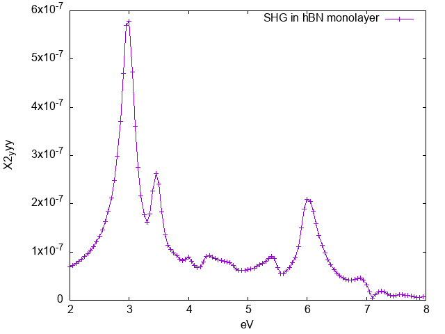
now you can plot columns 4 and 5 of the o.YPP-X_probe_order_2 file that are the real and imaginary part of Xhi2 along yyy direction. | |||
Using gnuplot, just plot | |||
p 'o.YPP-X_probe_order_2' u 1:(sqrt($4**2+$5**2)) t 'SHG in hBN monolayer' w lp | |||
and you will get | |||
[[File:Xhi2 hbn.png|center]] | |||
If you arrived up here, you have the right to listen to the [https://www.youtube.com/watch?v=gz2WMvHCJOU Yambo song]. | If you arrived up here, you have the right to listen to the [https://www.youtube.com/watch?v=gz2WMvHCJOU Yambo song]. | ||
== References == | == References == | ||
<references /> | <references> | ||
<ref name="Aryasetiawan1998"> F. Aryasetiawan, O. Gunnarsson, ''The '''GW''' method'', [https://doi.org/10.1088/0034-4885/61/3/002 Rep. Prog. Phys. '''61''', 237 (1998)]; ([https://arxiv.org/abs/cond-mat/9712013 arXiv 9712013]) </ref> | |||
<ref name="Gruning2016">M. Grüning, D. Sangalli, C. Attaccalite, ''Dielectrics in a time-dependent electric field: a real-time approach based on density-polarization functional theory'', [https://doi.org/10.1103/PhysRevB.94.035149 Phys. Rev. B '''94''', 035149 (2016)] </ref> | |||
<ref name="Martin1997">R. M. Martin and G. Ortiz, ''Functional theory of extended Coulomb systems'', [https://doi.org/10.1103/PhysRevB.56.1124 Phys. Rev. B '''56''', 1124 (1997)]</ref> | |||
<ref name="Botti">S. Botti, F. Sottile, N. Vast, V. Olevano, L. Reining, H. Weissker, A. Rubio, G. Onida, R. Del Sole, and R. W. Godby, ''Long-range contribution to the exchange-correlation kernel of time-dependent density functional theory'', [https://doi.org/10.1103/PhysRevB.69.155112 Phys. Rev. B '''69''', 155112 (2004)]</ref> | |||
<ref name="Attaccalite2011">C. Attaccalite, M. Grüning, and A. Marini, ''Real-time approach to the optical properties of solids and nanostructures: Time-dependent Bethe-Salpeter equation'', [https://doi.org/10.1103/PhysRevB.84.245110 Phys. Rev. B '''84''', 245110 (2011)]</ref> | |||
</references> | |||
==Links for schools== | |||
* Back to [[Rome 2023#Tutorials]] | |||
* Back to [[ICTP2020]] | |||
Latest revision as of 10:32, 23 January 2024
In this tutorial, we will show how to include correlation effects in the Second Harmonic Generation. We start from the tutorial on SHG in AlAs, using the same DFT inputs and parameters. Notice that the tutorials on TD-Hartree, TD-DFT, and TD-DPFT require more computational time, if calculations are too slow you can run in parallel or decrease the number of frequencies in your SHG.
Background
In real-time simulations using TDSE, correlation effects are determined by the choice of the Hamiltonian [math]\displaystyle{ H^{\text{sys}}_{\mathbf k} }[/math] that enters in the equations of motion(EOM).
Yambo can use different models for the system Hamiltonian:
- The independent-particle (IP) model,
[math]\displaystyle{ H^{\text{IP}}_{\mathbf k} \equiv H^{\text{KS}}_{\mathbf k} }[/math]
where [math]\displaystyle{ H^{\text{KS}}_{\mathbf k} }[/math] is the unperturbed KS Hamiltonian and we consider the KS system as a system of independent particles.
- The QP model,
[math]\displaystyle{ H^{\text{QP}}_{\mathbf k} \equiv H^{\text{KS}}_{\mathbf k} + \Delta H_{\mathbf k}. }[/math]
where [math]\displaystyle{ \Delta H_{\mathbf k} }[/math] is the GW correction or scissor operator, estimated from the Many-Body Perturbation Theory (Ref. [1]), and then applied to the KS eigenvalues.
- The RPA model (or Time-dependent Hartree),
[math]\displaystyle{ H^{\text{RPA}}_{\mathbf k} \equiv H^{\text{KS}}_{\mathbf k} + V_h(\mathbf r)[\Delta\rho], }[/math]
The term [math]\displaystyle{ V_h(\mathbf r)[\Delta\rho] }[/math] is the time-dependent Hartree potential and is responsible for the local-field effects originating from system inhomogeneities, and [math]\displaystyle{ \Delta \rho \equiv \rho(\mathbf r;t)-\rho(\mathbf r;t=0) }[/math] is the variation of the electronic density.
- The Time Dependent-Density Functional Theory (TD-DFT) model, at present only for LDA or GGA functionals:
[math]\displaystyle{ H^{\text{TDDFT}}_{\mathbf k} \equiv H^{\text{KS}}_{\mathbf k} + V_h(\mathbf r)[\Delta\rho] + V_{xc}(\mathbf r)[\Delta\rho] }[/math]
The term [math]\displaystyle{ V_{xc}(\mathbf r)[\Delta\rho] }[/math] is the time-dependent exchange-correlation potential.
- The Time Dependent-Density Polarization Function Theory (TD-DPFT) model, at present different functionals are implemented in Yambo, for more details see Ref. [2]:
[math]\displaystyle{ H^{\text{TD-DFTP}}_{\mathbf k} \equiv H^{\text{KS}}_{\mathbf k} + V_h(\mathbf r)[\Delta\rho] + V_{xc}(\mathbf r)[\Delta\rho] -\Omega \mathcal{E}^s(t) \cdot \nabla_{\mathbf k} }[/math]
where [math]\displaystyle{ \mathcal{E}^s(t) }[/math] is the Kohn-Sham macroscopic field (see Ref. [2], [3]).
Prerequisites
You need yambo_nl and ypp_nl compiled in double precision for this tutorial. You must have completed the previous tutorial on the non-linear response to do this one.
Quasi-particle corrections
Quasi-particle correction can be easily introduced in the real-time dynamics by means of a non-local operator that modifies the Kohn-Sham eigenvalues: [math]\displaystyle{ \Delta \hat H = \sum_{n,\bf k} \Delta_{n,\bf k} |v^0_{n,\bf k}\rangle\langle v^0_{n,\bf k}|. }[/math] The command to turn on quasi-particle corrections is: yambo_nl -u n -V qp :
nloptics                      # [R NL] Non-linear optics
% NLBands
  3 |  6 |                   # [NL] Bands
%
NLintegrator="INVINT"       # [NL] Integrator ("EULEREXP/RK4/RK2EXP/HEUN/INVINT/CRANKNIC")
NLCorrelation= "IPA"         # [NL] Correlation ("IPA/HARTREE/TDDFT/LRC/JGM/SEX/HF")
NLLrcAlpha= 0.000000         # [NL] Long Range Correction
% NLEnRange
 1.000000 | 5.000000 | eV    # [NL] Energy range
%
NLEnSteps= 5                # [NL] Energy steps
NLDamping= 0.150000    eV    # [NL] Damping
% Field1_Dir
 1.000000 | 1.000000 | 0.000000 |        # [RT Field1] Versor
%
Field1_kind= "SOFTSIN"         # [RT Field1] Kind(SIN|SOFTSIN|RES|ANTIRES|GAUSS|DELTA|QSSIN)
GfnQPdb= "none"              # [EXTQP G] Database
GfnQP_N= 1                   # [EXTQP G] Interpolation neighbours
% GfnQP_E
 0.900000 | 1.000000 | 1.000000 |        # [EXTQP G] E parameters  (c/v) eV|adim|adim
%
GfnQP_Z= ( 1.000000 , 0.000000 )       # [EXTQP G] Z factor  (c/v)
GfnQP_Wv_E= 0.000000   eV    # [EXTQP G] W Energy reference  (valence)
% GfnQP_Wv
 0.00     | 0.00     | 0.00     |        # [EXTQP G] W parameters  (valence) eV| eV|eV^-1
%
GfnQP_Wc_E= 0.000000   eV    # [EXTQP G] W Energy reference  (conduction)
% GfnQP_Wc
 0.00     | 0.00     | 0.00     |        # [EXTQP G] W parameters  (conduction) eV| eV|eV^-1
%
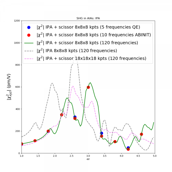
All the parameters of this input are the same of the previous tutorial with the only difference that we introduced a scissor operator of 0.9 eV. Notice that it is possible to import also the quasi-particle corrections calculated within the G0W0 approximation by using the flag GfnQPdb="E < SAVE/ndb.QP" (see Yambo tutorial on GW for more information). Now you can run Yambo and then analyze the results as explained in the previous tutorial. The effect of then scissor-operator is shown in the following figure:
The figure compares results with scissor operator "IPA + scissor" (red dots) with the one obtained in the previous tutorial "IPA". The full converged result is obtained with a 18x18x18 k-point grid and bands between 2 and 10 (violet dashed line). The script and the data to generate this plot can be downloaded here.
Time-dependent Hartree (RPA with local field effects)
In order to include local field effects in the SHG, we use the Time-dependent Hartree approximation. The input is generated with the usual command where we turned on the Reciprocal Lattice vectors verbosity in order to specify the number of plane waves to use in the calculations. To run a TD-Hartree calculation you just specify NLCorrelation="HARTREE" and then we reduce the number of plane waves to 105, that is enough to have a converged result in this system.
nloptics                      # [R NL] Non-linear optics
% NLBands
  3 |  6 |                   # [NL] Bands
%
NLintegrator="INVINT"       # [NL] Integrator ("EULEREXP/RK4/RK2EXP/HEUN/INVINT/CRANKNIC")
NLCorrelation= "HARTREE"         # [NL] Correlation ("IPA/HARTREE/TDDFT/LRC/JGM/SEX/HF")
NLLrcAlpha= 0.000000         # [NL] Long Range Correction
% NLEnRange
 1.000000 | 5.000000 | eV    # [NL] Energy range
%
NLEnSteps= 10                # [NL] Energy steps
HARRLvcs=  105         RL      # [HA] Hartree     RL components
EXXRLvcs=  105         RL      # [XX] Exchange    RL components
NLDamping= 0.250000    eV    # [NL] Damping
% ExtF_Dir
1.000000 | 1.000000 | 0.000000 | # [NL ExtF] Versor
%
ExtF_kind= "SOFTSIN"         # [NL ExtF] Kind(SIN|SOFTSIN|RES|ANTIRES|GAUSS|DELTA|QSSIN)
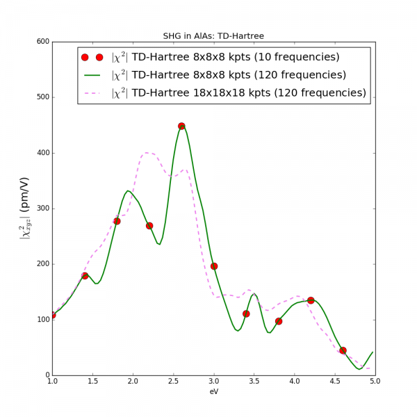
In this run we increase the damping to 0.25 eV in such a way to speed up calculations. The result of this calculation is shown in the figure below:
Plot data are available here.
Time-dependent Density Functional Theory (TD-DFT)
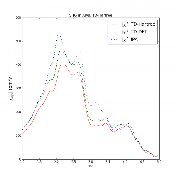
TD-DFT calculations are similar to the TD-Hartree ones. Just change NLCorrelation="TDDFT" and the exchange-correlation functional used in the ground state calculations will be included in the real-time dynamics. Notice that only LDA or GGA functionals are supported by Yambo/Lumen. These functionals usually provide insignificant improvement in respect to the TD-Hartree because they miss the long-range part that will be included in the next tutorial by means of TD-DPFT theory. You can perform TD-DFT calculations as exercise and compare them with the other approximations.
The converged result on a 18x18x18 k-points grid is reported below:
Plot data are available here.
Time-dependent Density-Polarization Functional Theory (TD-DPFT)
In this last tutorial on SHG we will include both quasi-particle effects by means of a scissor operator and long-range correction to the response function by means of Time-dependent Density-Polarization Functional Theory. The Lumen input can be generated as usual with the command yambo_nl -u n -V qp:
nloptics                      # [R NL] Non-linear optics
% NLBands
  3 | 6 |                   # [NL] Bands
%
NLintegrator="INVINT"       # [NL] Integrator ("EULEREXP/RK4/RK2EXP/HEUN/INVINT/CRANKNIC")
NLCorrelation= "LRC"     # [NL] Correlation ("IPA/HARTREE/TDDFT/LRC/JGM")
NLLrcAlpha= 0.350000         # [NL] Long Range Correction
% NLEnRange
 0.200000 | 8.000000 | eV    # [NL] Energy range
%
NLEnSteps= 10               # [NL] Energy steps
HARRLvcs=  105         RL      # [HA] Hartree     RL components
EXXRLvcs=  105         RL      # [XX] Exchange    RL components
NLDamping= 0.150000    eV    # [NL] Damping
% ExtF_Dir
 1.000000 | 1.000000 | 0.000000 |        # [RT Field1] Versor
%
Field1_kind= "SOFTSIN"         # [RT Field1] Kind(SIN|SOFTSIN|RES|ANTIRES|GAUSS|DELTA|QSSIN)
GfnQPdb= "none"              # [EXTQP G] Database
GfnQP_N= 1                   # [EXTQP G] Interpolation neighbours
% GfnQP_E
 0.900000 | 1.000000 | 1.000000 |        # [EXTQP G] E parameters  (c/v) eV|adim|adim
%
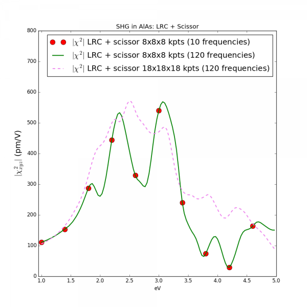
The [math]\displaystyle{ \alpha }[/math] parameter for AlAs has been taken from Ref. [4]. The results is:
Plot data are available here. Notice that different models for the \( \alpha \) parameter have been proposed in the literature, see Ref. [2] for a discussion. Finally, in Yambo we implemented also the Jelium-with gap model NLCorrelation="JGM" that provides an automatic estimation of the \( \alpha \) parameters for each material, see Ref. [2] for a discussion on this approximation.
SHG at the TD-BSE level
Second-harmonic generation can be calculated also the TD-BSE level, the procedure is the same of the linear response case: the first one has to calculate the collisions integrals (see appendix of Ref.[5]) and then can run simulation for the non-linear response as it is shown in this tutorial. Hereafter we will briefly repeat the steps necessary to obtain SHG including excitonic effects.
1) Download DFT wave-functions and input file here: hBN-2D-RT.tar.gz
2) Run the setup
3) Remove symmetries
use the command ypp_nl -y
fixsyms
# [R] Remove symmetries not consistent with an external perturbation
% Efield1
  0.000000 | 1.000000 | 0.000000 |        # First external Electric Field
%
% Efield2
 0.000000 | 0.000000 | 0.000000 |        # Additional external Electric Field
%
BField= 0.000000           T     # [MAG] Magnetic field modulus
Bpsi= 0.000000             deg   # [MAG] Magnetic field psi angle [degree]
Btheta= 0.000000           deg   # [MAG] Magnetic field theta angle [degree]
RmTimeRev                     # Remove Time Reversal
then go in the FixSymm folder and run the setup again
4) Generate collisions integrals generate collision for HSEX using the command: yambo_nl -X s -e -v h+sex
em1s                             # [R][Xs] Statically Screened Interaction
collisions                       # [R] Collisions
dipoles                          # [R] Oscillator strenghts (or dipoles)
DIP_Threads=0                    # [OPENMP/X] Number of threads for dipoles
X_Threads=0                      # [OPENMP/X] Number of threads for response functions
RT_Threads=0                     # [OPENMP/RT] Number of threads for real-time
Chimod= "HARTREE"                # [X] IP/Hartree/ALDA/LRC/PF/BSfxc
% BndsRnXs
  1 | 20 |                       # [Xs] Polarization function bands
%
 NGsBlkXs= 3000 mHa              # [Xs] Response block size
% LongDrXs
 1.000000 | 0.000000 | 0.000000 |        # [Xs] [cc] Electric Field
%
% COLLBands
  4 | 5 |                           # [COLL] Bands for the collisions
%
HXC_Potential= "SEX+HARTREE"     # [SC] SC HXC Potential
HARRLvcs= 1000             mHa    # [HA] Hartree     RL components
EXXRLvcs= 1000             mHa    # [XX] Exchange    RL components
CORRLvcs= 1000             mHa    # [GW] Correlation RL components
5) Run the SHG calculation including collisions, with the command: yambo_nl -u n -V qp
nloptics                         # [R] Non-linear spectroscopy
DIP_Threads=0                    # [OPENMP/X] Number of threads for dipoles
NL_Threads=0                     # [OPENMP/NL] Number of threads for nl-optics
% NLBands
  4 |  5 |                           # [NL] Bands range
%
NLverbosity= "high"              # [NL] Verbosity level (low | high)
NLtime=42.000000          fs    # [NL] Simulation Time
NLintegrator= "CRANKNIC"         # [NL] Integrator ("EULEREXP/RK2/RK4/RK2EXP/HEUN/INVINT/CRANKNIC")
NLCorrelation= "SEX"             # [NL] Correlation ("IPA/HARTREE/TDDFT/LRC/LRW/JGM/SEX")
NLLrcAlpha= 0.000000             # [NL] Long Range Correction
% NLEnRange
  2.000000 | 8.000000 |         eV    # [NL] Energy range
%
NLEnSteps=  80                   # [NL] Energy steps
NLDamping= 0.200000        eV    # [NL] Damping (or dephasing)
RADLifeTime=-1.000000      fs    # [RT] Radiative life-time (if negative Yambo sets it equal to Phase_LifeTime in NL)
#EvalCurrent                   # [NL] Evaluate the current
#FrPolPerdic                   # [DIP] Force periodicity of polarization respect to the external field
HARRLvcs= 1000             mHa   # [HA] Hartree     RL components
EXXRLvcs= 1000             mHa   # [XX] Exchange    RL components
GfnQPdb= "none"                  # [EXTQP G] Database action
GfnQP_INTERP_NN= 1               # [EXTQP G] Interpolation neighbours (NN mode)
GfnQP_INTERP_shells= 20.00000    # [EXTQP G] Interpolation shells (BOLTZ mode)
GfnQP_DbGd_INTERP_mode= "NN"     # [EXTQP G] Interpolation DbGd mode
% GfnQP_E
   3.000000 | 1.000000 | 1.000000 |        # [EXTQP G] E parameters  (c/v) eV|adim|adim
%
.............
% Field1_Freq
 0.100000 | 0.100000 |         eV    # [RT Field1] Frequency
%
Field1_NFreqs= 1                 # [RT Field1] Frequency
Field1_Int=  1000.00       kWLm2 # [RT Field1] Intensity
Field1_Width= 0.000000     fs    # [RT Field1] Width
Field1_kind= "SOFTSIN"           # [RT Field1] Kind(SIN|COS|RES|ANTIRES|GAUSS|DELTA|QSSIN)
Field1_pol= "linear"         # [RT Field1] Pol(linear|circular)
% Field1_Dir
 0.000000 | 1.000000 | 0.000000 |        # [RT Field1] Versor
%
6) Use the command ypp_nl -u to analyze the result
nonlinear                        # [R] Non-linear response analysis
Xorder= 4                        # Max order of the response/exc functions
% TimeRange
 40.000 | -1.00000 |         fs    # Time-window where processing is done
%
ETStpsRt= 200                    # Total Energy steps
% EnRngeRt
  0.00000 | 20.00000 |         eV    # Energy range
%
DampMode= "NONE"                 # Damping type ( NONE | LORENTZIAN | GAUSSIAN )
DampFactor= 0.000000       eV    # Damping parameter
PumpPATH= "none"                 # Path of the simulation with the Pump only
now you can plot columns 4 and 5 of the o.YPP-X_probe_order_2 file that are the real and imaginary part of Xhi2 along yyy direction. Using gnuplot, just plot
p 'o.YPP-X_probe_order_2' u 1:(sqrt($4**2+$5**2)) t 'SHG in hBN monolayer' w lp
and you will get
If you arrived up here, you have the right to listen to the Yambo song.
References
- ↑ F. Aryasetiawan, O. Gunnarsson, The GW method, Rep. Prog. Phys. 61, 237 (1998); (arXiv 9712013)
- ↑ 2.0 2.1 2.2 2.3 M. Grüning, D. Sangalli, C. Attaccalite, Dielectrics in a time-dependent electric field: a real-time approach based on density-polarization functional theory, Phys. Rev. B 94, 035149 (2016)
- ↑ R. M. Martin and G. Ortiz, Functional theory of extended Coulomb systems, Phys. Rev. B 56, 1124 (1997)
- ↑ S. Botti, F. Sottile, N. Vast, V. Olevano, L. Reining, H. Weissker, A. Rubio, G. Onida, R. Del Sole, and R. W. Godby, Long-range contribution to the exchange-correlation kernel of time-dependent density functional theory, Phys. Rev. B 69, 155112 (2004)
- ↑ C. Attaccalite, M. Grüning, and A. Marini, Real-time approach to the optical properties of solids and nanostructures: Time-dependent Bethe-Salpeter equation, Phys. Rev. B 84, 245110 (2011)
Links for schools
- Back to Rome 2023#Tutorials
- Back to ICTP2020
| Prev: Non Linear Response | Now: ICTP Tutorials --> Correlation effects in the non-linear response |
