How to obtain the quasi-particle band structure of a bulk material: h-BN
In this tutorial you will learn how to:
- Calculate quasi-particle corrections in the Hartree-Fock approximation
- Calculate quasi-particle corrections in the GW approximation
- Choose the input parameters for a meaningful converged calculation
- Plot a band structure including quasi-particle corrections
We will use bulk hBN as an example system. Before starting, you need to obtain the appropriate tarball. See instructions on the main tutorials page.
We strongly recommend that you first complete the First steps: a walk through from DFT to optical properties tutorial.
The aim of the present tutorial is to obtain quasiparticle correction to energy levels using many-body perturbation theory (MBPT).
The general non-linear quasiparticle equation reads:
As a first step we want to evaluate the self energy Σ entering in the quasiparticle equation. In the GW approach the self-energy can be separated into two components: a static term called the exchange self-energy (Σx), and a dynamical term (energy dependent) called the correlation self-energy (Σc):
We will treat these two terms separately and demonstrate how to set the most important variables for calculating each term. In practice we will compute the quasi-particle corrections to the one particle Kohn-Sham eigenvalues obtained through a DFT calculation.
The steps are the following:
Step 1: The Exchange Self Energy or HF quasi-particle correction
We start by evaluating the exchange Self-Energy and the corresponding Quasiparticle energies (Hartree-Fock energies). Follow the module on Hartree Fock and then return to this tutorial How to obtain the quasiparticle band structure of a bulk material: h-BN.
Step 2: The Correlation Self-Energy and Quasiparticle Energies
Once we have calculated the exchange part, we next turn our attention to the more demanding dynamical part. The correlation part of the self-energy in a plane wave representation reads:

In the expression for the correlation self energy, we have (1) a summation over bands, (2) an integral over the Brillouin Zone, and (3) a sum over the G vectors. In contrast with the case of Σx, the summation over bands extends over all bands (including the unoccupied ones), and so convergence tests are needed. Another important difference is that the Coulomb interaction is now screened so a fundamental ingredient is the evaluation of the dynamical dielectric matrix. The expression for the dielectric matrix, calculated at the RPA level and including local field effects, has been already treated in the Local fields tutorial.
In the following, we will see two ways to take into account the dynamical effects. First, we will see how to set the proper parameters to obtain a model dielectric function based on a widely used approximation, which models the energy dependence of each component of the dielectric matrix with a single pole function. Secondly, we will see how to perform calculations by evaluating the dielectric matrix on a regular grid of frequencies.
Once the correlation part of the self-energy is calculated, we will check the convergence of the different parameters with respect to some final quantity, such as the gap.
After computing the frequency dependent self-energy, we will discover that in order to solve the quasiparticle equation we will need to know its value at the value of the quasiparticle itself. In the following, unless explicitly stated, we will solve the non-linear quasi-particle equation at first order, by expanding the self-energy around the Kohn-Sham eigenvalue. In this way the quasiparticle equation reads:
where the normalization factor Z is defined as:
The Plasmon Pole approximation
As stated above, the basic idea of the plasmon-pole approximation is to approximate the frequency dependence of the dielectric matrix with a single pole function of the form:
The two parameters RGG' and ΩGG' are obtained by a fit (for each component), after having calculated the RPA dielectric matrix at two given frequencies. Yambo calculates the dielectric matrix in the static limit ( ω=0) and at a user defined frequency called the plasmon-pole frequency (ω=iωp). Such an approximation has the big computational advantage of calculating the dielectric matrix for only two frequencies and leads to an analytical expression for the frequency integral of the correlation self-energy.
Input file generation
Let's start by building up the input file for a GW/PPA calculation, including the calculation of the exchange self-energy. From yambo -H you should understand that the correct option is yambo -x -p p -g n:
$ cd YAMBO_TUTORIALS/hBN/YAMBO
$ yambo -x -p p -g n -F gw_ppa.in
Let's modify the input file in the following way:
HF_and_locXC                 # [R XX] Hartree-Fock Self-energy and Vxc
ppa                          # [R Xp] Plasmon Pole Approximation
gw0                          # [R GW] GoWo Quasiparticle energy levels
em1d                         # [R Xd] Dynamical Inverse Dielectric Matrix
EXXRLvcs = 40         Ry    # [XX] Exchange RL components
VXCRLvcs = 3187        RL      # [XC] XCpotential RL components
Chimod= "Hartree"                   # [X] IP/Hartree/ALDA/LRC/BSfxc
% BndsRnXp
  1 | 10 |                 # [Xp] Polarization function bands
%
NGsBlkXp= 1000          mRy    # [Xp] Response block size
% LongDrXp
 1.000000 | 1.000000 | 1.000000 |        # [Xp] [cc] Electric Field
%
PPAPntXp = 27.21138     eV    # [Xp] PPA imaginary energy
%GbndRnge
  1 | 40 |                 # [GW] G[W] bands range
%
GDamping=  0.10000     eV    # [GW] G[W] damping
dScStep=  0.10000      eV    # [GW] Energy step to evaluate Z factors
DysSolver= "n"               # [GW] Dyson Equation solver ("n","s","g")
%QPkrange        # [GW] QP generalized Kpoint/Band indices
 7|  7|  8|  9|
%
Brief explanation of some settings:
- Similar to the Hartree Fock study, we will concentrate on the convergence of the direct gap of the system. Hence we select the last occupied (8) and first unoccupied (9) bands for k-point number 7 in the
QPkrangevariable. - We also keep
EXXRLvcsat its converged value of 40 Ry as obtained in the Hartree Fock tutorial. - For the moment we keep fixed the plasmon pole energy
PPAPntXpat its default value (=1 Hartree). - We keep fixed the direction of the electric field for the evaluation of the dielectric matrix to a non-specific value:
LongDrXp=(1,1,1). - Later we will study convergence with respect to
GbndRnge,NGsBlkXp, andBndsRnXp; for now just set them to the values indicated.
Understanding the output
Let's look at the typical Yambo output. Run Yambo with an appropriate -J flag:
$ yambo -F gw_ppa.in -J 10b_1Ry
In the standard output you can recognise the different steps of the calculations: calculation of the screening matrix (evaluation of the non interacting and interacting response), calculation of the exchange self-energy, and finally the calculation of the correlation self-energy and quasiparticle energies. Moreover information on memory usage and execution time are reported:
...
<---> [05] Dynamic Dielectric Matrix (PPA)
...
<08s> Xo@q[3] |########################################| [100%] 03s(E) 03s(X)
<08s> X@q[3] |########################################| [100%] --(E) --(X)
...
<43s> [06] Bare local and non-local Exchange-Correlation
<43s> EXS |########################################| [100%] --(E) --(X)
...
<43s> [07] Dyson equation: Newton solver
<43s> [07.01] G0W0 (W PPA)
...
<45s> G0W0 (W PPA) |########################################| [100%] --(E) --(X)
...
<45s> [07.02] QP properties and I/O
<45s> [08] Game Over & Game summary
Let's have a look at the report and output. The output file o-10b_1Ry.qp contains (for each band and k-point that we indicated in the input file) the values of the bare KS eigenvalue, its GW correction and the correlation part of the self energy:
#
#  K-point    Band       Eo         E-Eo       Sc|Eo
#
 7.000000   8.000000  -0.411876  -0.567723   2.322443
 7.000000   9.000000   3.877976   2.413773  -2.232241
In the header you can see the details of the calculations, for instance it reports that NGsBlkXp=1 Ry corresponds to 5 Gvectors:
# X G`s [used]: 5
Other information can be found in the report file r-10b_1Ry_em1d_ppa_HF_and_locXC_gw0, such as the renormalization factor defined above, the value of the exchange self-energy (non-local XC) and of the DFT exchange-correlation potential (local XC):
[07.02] QP properties and I/O
 =============================
 Legend (energies in eV):
 - B  : Band       - Eo  : bare energy
 - E  : QP energy  - Z   : Renormalization factor
 - So : Sc(Eo)     - S   : Sc(E)
 - dSp: Sc derivative precision
 - lXC: Starting Local XC (DFT)
 -nlXC: Starting non-Local XC (HF)
 QP [eV] @ K [7] (iku): 0.000000 -0.500000  0.000000
  B=8 Eo= -0.41 E= -0.98 E-Eo= -0.56 Re(Z)=0.81 Im(Z)=-.2368E-2 nlXC=-19.13 lXC=-16.11 So= 2.322
  B=9 Eo=  3.88 E=  6.29 E-Eo=  2.41 Re(Z)=0.83 Im(Z)=-.2016E-2 nlXC=-5.536 lXC=-10.67 So=-2.232
Extended information can be also found in the output activating in the input the ExtendOut flag. This is an optional flag that can be activated by adding the -V qp verbosity option when building the input file. The plasmon pole screening, exchange self-energy and the quasiparticle energies are also saved in databases so that they can be reused in further runs:
$ ls ./10b_1Ry
ndb.pp ndb.pp_fragment_1 ... ndb.HF_and_locXC ndb.QP
Convergence tests for a quasi particle calculation
Now we can check the convergence of the different variables entering in the expression of the correlation part of the self energy.
First, we focus on the parameter governing the screening matrix you have already seen in the RPA/IP section. In contrast to the calculation of the RPA/IP dielectric function, where you considered either the optical limit or a finite q response (EELS), here the dielectric matrix will be calculated for all q-points determined by the choice of k-point sampling.
The parameters that need to be converged can be understood by looking at expression of the dielectric matrix:
where χGG' is given by
and χ0GG' is given by
NGsBlkXp: The dimension of the microscopic inverse matrix, related to Local fieldsBndsRnXp: The sum on bands (c,v) in the independent particle χ0GG'
Converging Screening Parameters
Here we will check the convergence of the gap starting from the variables controlling the screening reported above: the bands employed to build the RPA response function BndsRnXp and the number of blocks (G,G') of the dielectric matrix ε-1G,G' NGsBlkXp.
In the next section we will study convergence with respect to the sum over states summation (sum over m in the Σc expression); here let's fix GbndRnge to a reasonable value (40 Ry).
Let's build a series of input files differing by the values of bands and block sizes in χ0GG' considering BndsRnXp in the range 10-50 (upper limit) and NGsBlkXp in the range 1000 to 5000 mRy. To do this by hand, file by file, open the gw_ppa.in file in an editor and change to:
NGsBlkXp = 2000 mRy
while leaving the rest untouched. Repeat for 3000 mRy, 4000 mRy etc. Next, for each NGsBlkXp change to:
% BndsRnXp
  1 | 20 |                 # [Xp] Polarization function bands
%
and repeat for 30, 40 and so on. Give a different name to each file: gw_ppa_Xb_YRy.in with X=10,20,30,40 and Y=1000,2000,3000,4000,5000 mRy.
This is obviously quite tedious. However, you can automate both the input construction and code execution using bash or python scripts (indeed later you will learn how to use the the yambo-python [1]tool for this task). For now, you can use the simple generate_inputs_1.sh bash script to generate the required input files (after copying the script you need to type $ chmod +x name_of_the_script.sh ).
Finally launch the calculations:
$ yambo -F gw_ppa_10b_1Ry.in -J 10b_1Ry
$ yambo -F gw_ppa_10b_2Ry.in -J 10b_2Ry
...
$ yambo -F gw_ppa_40b_5Ry.in -J 40b_5Ry
Once the jobs are terminated we can collect the quasiparticle energies for fixed BndsRnXp in different files named e.g. 10b.dat, 20b.dat etc. for plotting, by putting in separate columns: the energy cutoff; the size of the G blocks; the quasiparticle energy of the valence band; and that of the conduction band.
To do this e.g. for the 10b.dat file you can type:
$ cat o-10b* | grep "8.000" | awk '{print $3+$4}'
to parse the valence band quasiparticle energies and
$ cat o-10b* | grep "9.000" | awk '{print $3+$4}'
for the conduction band; and put all the data in the 10b.dat files. As there are many files to process you can use the parse_qps.sh script to create the 10b.dat file and edit the script changing the number of BndsRnXp for the other output files.
Once we have collected all the quasiparticle values we can plot the gap, or the valence and conduction band energies separately, as a function of the block size or energy cutoff:
$ gnuplot
gnuplot> p "10b.dat" u 1:3 w lp t " Valence BndsRnXp=10", "20b.dat" u 1:3 w lp t "Valence BndsRnXp=20",..
gnuplot> p "10b.dat" u 1:4 w lp t " Conduction BndsRnXp=10", "20b.dat" u 1:4 w lp t "Conduction BndsRnXp=20",..
gnuplot> p "10b.dat" u 1:($4-$3) w lp t " Gap BndsRnXp=10", "20b.dat" u 1:($4-$3) w lp t "gap BndsRnXp=20",..
or both using e.g. the ppa_gap.gnu gnuplot script:
- Quasiparticle energies with respect screening parameters


Looking at the plot we can see that:
- The two parameters are not totally independent (see e.g. the valence quasiparticle convergence) and this is the reason why we converged them simultaneously
- The gap (energy difference) converge faster than single quasiparticle state
- The convergence criteria depends on the degree of accuracy we look for, but considering the approximations behind the calculations (plasmon-pole etc.), it is not always a good idea to enforce too strict a criteria.
- Even if not totally converged we can consider that the upper limit of
BndsRnXp=30, andNGsBlkXp=3Ry are reasonable parameters.
Finally notice that in the last versions of Yambo 4.5 etc. there is a terminator for the dielectric constant that accelerates convergence on the number of bands,
you can active it with the -V resp verbosity and setting XTermKind= "BG". You can compare the converge of the dielectric constant with and without terminator,
similar to what happens for the self-energy, see next section.
Converging the sum over states in the correlation self-energy
From now on we will keep fixed these parameters and will perform a convergence study on the sum over state summation in the correlation self-energy (Σc) GbndRnge.
In order to use the screening previously calculated we can copy the plasmon pole parameters saved in the 30b_3Ry directory in the SAVE directory. In this way the screening will be read by Yambo and not calculated again:
$ cp ./30b_3Ry/ndb.pp* ./SAVE/.
(Note: you may have to delete these files before running the BSE tutorials)
In order to use the databases we have to be sure to have the same plasmon-pole parameters in our input files.
Edit gw_ppa_30b_3Ry.in and modify GbndRnge to order to have a number of bands in the range from 10 to 80 inside different files named gw_ppa_Gbnd10.in, gw_ppa_Gbnd20.in etc. You can also run the the generate_inputs_2.sh bash script to generate the required input files.
Next, launch yambo for each input:
$ yambo -F gw_ppa_Gbnd10.in -J Gbnd10
$ yambo -F gw_ppa_Gbnd20.in -J Gbnd20
...
and as done before we can inspect the obtained quasiparticle energies:
$ grep 8.00 o-Gbnd* | awk '{print $4+$5}'
for the valence bands, and
$ grep 9.00 o-Gbnd* | awk '{print $4+$5}'
for the conduction band.
Collect the results in a text file Gbnd_conv.dat containing: the number of Gbnd, the valence energy, and the conduction energy. Now, as done before we can plot the valence and conduction quasiparticle levels separately as well as the gap, as a function of the number of bands used in the summation:
$ gnuplot
gnuplot> p "Gbnd_conv.dat" u 1:2 w lp lt 7  t "Valence"
gnuplot> p "Gbnd_conv.dat" u 1:3 w lp lt 7  t "Conduction"
gnuplot> p "Gbnd_conv.dat" u 1:($3-$2) w lp lt 7  t "Gap"
- Quasiparticle energies with respect sum over states in correlation self-energy
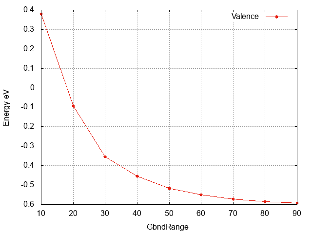
Valence band energy wrt
GbndRange.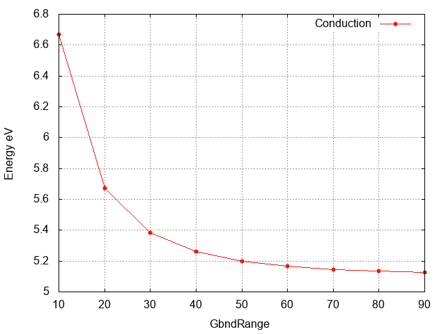
Conduction band energy wrt
GbndRange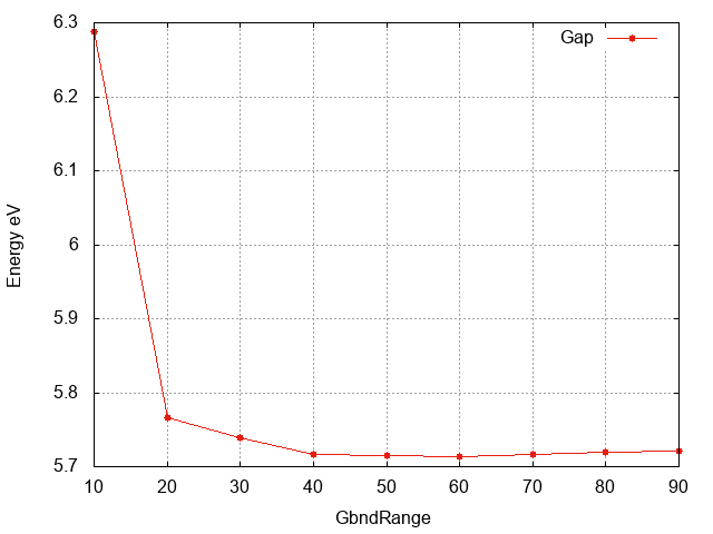
Gap energy wrt
GbndRange


Inspecting the plot we can see that:
- The convergence with respect to
GbndRangeis rather slow and many bands are needed to get converged results. - As observed above the gap (energy difference) converges faster than the single quasiparticle state energies.
Accelerating the sum over states convergence in the correlation self-energy
In general the convergence with respect the sum over states can be very cumbersome. Here we show how it can be mitigated by using a technique developed by F. Bruneval and X. Gonze [1]. The basic idea relies in replacing the eigenenergies of the states that are not treated explicitly by a common energy, and take into account all the states, which are not explicitly included in the calculation through the closure relation. To apply this technique in Yambo we need to activate the optional terminator variable GTermKind. We can activate it by adding the quasiparticle verbosity to the command line when generating the input file:
$ yambo -p p -g n -F gw_ppa_Gbnd10.in -V qp
and you can edit the input file by setting:
GTermKind= "BG"
or simply you can add by hand this line in all the other gw_ppa_GbndX.in input files. Now we can repeat the same calculations
$ yambo -F gw_ppa_Gbnd10.in -J Gbnd10_term
$ yambo -F gw_ppa_Gbnd20.in -J Gbnd20_term
...
and collect the new results:
$ grep 8.000 *term.qp  | awk '{print $4+$5}'
$ grep 9.000 *term.qp  | awk '{print $4+$5}'
in a new file called Gbnd_conv_terminator.dat. Now we can plot the same quantities as before by looking at the effect of having introduced the terminator.
gnuplot
gnuplot> p "Gbnd_conv.dat" u 1:2  w lp t "Valence", "Gbnd_conv_terminator.dat" u 1:2 w lp t "Valence with terminator"
gnuplot> p "Gbnd_conv.dat" u 1:3  w lp t "Conduction", "Gbnd_conv_terminator.dat" u 1:3 w lp t "Conduction with terminator"
gnuplot> p "Gbnd_conv.dat" u 1:($3-$2)  w lp t "Gap", "Gbnd_conv_terminator.dat" u 1:($3-$2) w lp t "Gap with terminator"
- Effect of the terminator in convergence of QP energies with respect sum over states
![Valence band energy wrt GbndRange with and without the terminator technique [1]](/wiki/index.php?title=File:Val_t.png)
![Conduction band energy wrt GbndRange with and without the terminator technique[1]](/wiki/index.php?title=File:Cond_t.png)
![Gap energy wrt GbndRange with and without the terminator technique[1]](/wiki/index.php?title=File:Gap_t.png)
We can see that:
- The convergence with respect to
GbndRangeis accelerated in particular for the single quasiparticle states. - From the plot above we can see that
GbndRange=40 is sufficient to have a converged gap
Beyond the plasmon pole approximation: a full frequency approach - real axis integration
All the calculations performed up to now were based on the plasmon pole approximation (PPA). Now we remove this approximation by evaluating numerically the frequency integral in the expression of the correlation self-energy (Σc). To this aim we need to evaluate the screening for a number of frequencies in the interval depending on the electron-hole energy difference (energy difference between empty and occupied states) entering in the sum over states. Let's build the input file for a full frequency calculation by simply typing:
$ yambo -F gw_ff.in -g n
and we can set the variable studied up to now at their converged value:
%BndsRnXd
1 | 30 |
%
NGsBlkXd=3000 mRy
%GbndRange
1 | 40 |
%
EXXRLvcs=40000 mRy
% LongDrXd
1.000000 | 1.000000 | 1.000000 |        # [Xd] [cc] Electric Field
%
%QPkrange                      # # [GW] QP generalized Kpoint/Band indices
7|7|8|9|
%
and next vary in different files (name them gw_ff10.in etc.) the number of frequencies we evaluate for the screened coulomb potential. This is done by setting the values of ETStpsXd=10 , 50 , 100, 150, 200, 250.
You can also run the the generate_inputs_3.sh bash script to generate the required input files.
Next launch yambo:
$ yambo -F gw_ff10.in -J ff10
$ yambo -F gw_ff50.in -J ff50
...
Clearly as we are evaluating the screening for a large number of frequencies these calculations will be heavier than the case above where the calculation of the screening was done for only two frequencies (zero and plasmon-pole). As before, collect the valence and conduction bands as a function of the number of frequencies in a file called gw_ff.dat and plot the behaviour of the conduction and valence bands and the gap.
$ gnuplot
gnuplot> p "gw_ff.dat" u 1:2  w lp t "Valence"
gnuplot> p "gw_ff.dat" u 1:3  w lp t "Conduction"
gnuplot> p "gw_ff.dat" u 1:($3-$2)  w lp t "Gap"
- Real axis integration, convergences with respect the used number of frequencies

Valence band energy wrt
ETStpsXd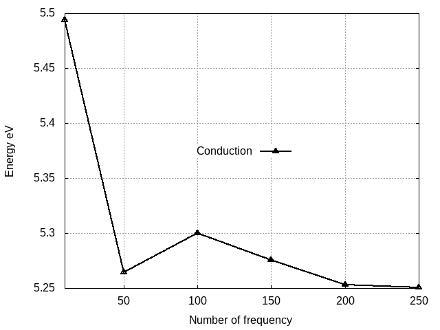
Conduction band energy wrt
ETStpsXd
Gap energy wrt
ETStpsXd


We can see that:
- Oscillations are still present, indicating that even more frequencies have to be considered. In general, a real-axis calculation is very demanding.
- The final result of the gap obtained up to now does not differ too much from the one obtained at the plasmon-pole level (~50 meV)
Secant Solver
The real axis integration permits also to go beyond the linear expansion to solve the quasi particle equation. The QP equation is a non-linear equation whose solution must be found using a suitable numerical algorithm.
The mostly used, based on the linearization of the self-energy operator is the Newton method that is the one we have used up to now. Yambo can also perform a search of the QP energies using a non-linear iterative method based on the Secant iterative Method.
In numerical analysis, the secant method is a root-finding algorithm that uses a succession of roots of secant lines to better approximate a root of a function f. The secant method can be thought of as a finite difference approximation of Newton's method. The equation that defines the secant method is:
The first two iterations of the secant method are shown in the following picture. The red curve shows the function f and the blue lines are the secants.

To see if there is any non-linear effect in the solution of the Dyson equation we compare the result of the calculation using the Newton solver as done before with the present case. In order to use the secant method you need to edit one of the the previous gw_ffN.in files e.g. gw_ff100.in and substitute:
DysSolver= "g"
to
DysSolver= "s"
Repeat the calculations in the same way as before:
$ yambo -F gw_ff100.in -J ff100
Note than now the screening will not be calculated again as it has been stored in the ffN directories as can be seen in the report file:
[05] Dynamical Dielectric Matrix
================================
[RD./ff10//ndb.em1d]----
...
[RD./ff10//ndb.em1d_fragment_1]--------------
...
Comparing the output files, e.g. for the case with 100 freqs:
o-ff100.qp Newton Solver:
#  K-point    Band       Eo         E-Eo       Sc|Eo
#
  7.00000   8.00000   -0.41188   -0.08708      2.91254
  7.00000   9.00000   3.877976   1.421968    -3.417357
o-ff100.qp_01 Secant Solver:
#
#  K-point    Band       Eo         E-Eo       Sc|Eo
#
  7.00000   8.00000   -0.41188   -0.08715      2.93518
  7.00000   9.00000   3.877976   1.401408    -3.731649
From the comparison, we see that the effect is of the order of 20 meV, of the same order of magnitude of the accuracy of the GW calculations.
Step 3: Interpolating Band Structures
Up to now we have checked convergence for the gap. Now we want to calculate the quasiparticle corrections across the Brillouin zone in order to visualize the entire band structure along a path connecting high symmetry points.
To do that we start by calculating the QP correction in the plasmon-pole approximation for all the k points of our sampling and for a number of bands around the gap. You can use a previous input file or generate a new one: yambo -F gw_ppa_all_Bz.in -x -p p -g n and set the parameters found in the previous tests:
EXXRLvcs=  40        Ry
% BndsRnXp
  1 | 30 |                 # [Xp] Polarization function bands
%
NGsBlkXp= 3000            mRy    # [Xp] Response block size
% LongDrXp
 1.000000 | 1.000000 | 1.000000 |        # [Xp] [cc] Electric Field
%
PPAPntXp= 27.21138     eV    # [Xp] PPA imaginary energy
% GbndRnge
  1 | 40 |                 # [GW] G[W] bands range
%
and we calculate it for all the available kpoints by setting:
%QPkrange                    # [GW] QP generalized Kpoint/Band indices
 1| 14|  6|11|
%
Note that as we have already calculated the screening with these parameters you can save time and use that database either by running in the previous directory by using -J 30b_3Ry or if you prefer to put the new databases in the new all_Bz directory you can create a new directory and copy there the screening databases:
$ mkdir all_Bz
$ cp ./30b_3Ry/ndb.pp* ./all_Bz/
and launch the calculation:
$ yambo -F gw_ppa_all_Bz.in -J all_Bz
Now we can inspect the output and see that it contains the correction for all the k points for the bands we asked:
#  K-point    Band       Eo         E-Eo       Sc|Eo
#
   1.000000     6.000000    -1.299712    -0.219100     3.788044
   1.000000     7.000000    -1.296430    -0.241496     3.788092
   1.000000     8.000000    -1.296420    -0.243115     3.785947
   1.000000     9.000000     4.832399     0.952386    -3.679259
   1.00000     10.00000     10.76416      2.09915     -4.38743
   1.00000     11.00000     11.36167      2.48053     -3.91021
.... By plotting some of the 'o-all_Bz.qp" columns it is possible to discuss some physical properties of the hBN QPs. Using columns 3 and (3+4), ie plotting the GW energies with respect to the LDA energies we can deduce the band gap renormalization and the stretching of the conduction/valence bands:
$ gnuplot
gnuplot> p "o-all_Bz.qp" u 3:($3+$4) w p  t "Eqp vs Elda"

Essentially we can see that the effect of the GW self-energy is the opening of the gap and a linear stretching of the conduction/valence bands that can be estimated by performing a linear fit of the positive and negative energies (the zero is set at top of the valence band).
In order to calculate the band structure, however, we need to interpolate the values we have calculated above on a given path. In Yambo the interpolation is done by the executable ypp (Yambo Post Processing).
By typing:
$ ypp -H
you will recognize that in order to interpolate the bands we need to build a ypp input file using
$ ypp -s b
we can generate the input for the band interpolation:
$ypp -s b -F ypp_bands.in
and edit the ypp_bands.in file:
electrons                    # [R] Electrons (and holes)
bnds                         # [R] Bands
INTERP_mode= "NN"              # Interpolation mode (NN=nearest point, BOLTZ=boltztrap aproach)
OutputAlat= 4.716000           # [a.u.] Lattice constant used for "alat" ouput format
cooIn= "rlu"                   # Points coordinates (in) cc/rlu/iku/alat
cooOut= "rlu"
% BANDS_bands
  1 | 100 |                   # Number of bands
%
% INTERP_Grid
-1 |-1 |-1 |                             # Interpolation BZ Grid
%
INTERP_Shell_Fac= 20.00000     # The bigger it is a higher number of shells is used
CIRCUIT_E_DB_path= "none"      # SAVE obtained from the QE `bands` run (alternative to %BANDS_kpts)
BANDS_path= ""                 # BANDS path points labels (G,M,K,L...)
BANDS_steps= 10
#BANDS_built_in                # Print the bands of the generating points of the circuit using the nearest internal point
%BANDS_kpts
%
We modify the following lines:
BANDS_steps=30
% BANDS_bands
  6 | 11 |                   # Number of bands
%
%BANDS_kpts                    # K points of the bands circuit
 0.33300 |-.66667 |0.00000 |
 0.00000 |0.00000 |0.00000 |
 0.50000 |-.50000 |0.00000 |
 0.33300 |-.66667 |0.00000 |
 0.33300 |-.66667 |0.50000 |
 0.00000 |0.00000 |0.50000 |
 0.50000 |-.50000 |0.50000 |
%
which means we assign 30 points in each segment, we ask to interpolate 3 occupied and 3 empty bands and we assign the following path passing from the high symmetry points: K Γ M K H A L. Launching:
$ ypp -F ypp_bands.in
will produce the output file o.bands_interpolated containing:
#
#   |k|        b6         b7         b8         b9         b10        b11        kx         ky         kz
#
#
    0.00000   -7.22092   -0.13402   -0.13395    4.67691    4.67694   10.08905    0.33300   -0.66667    0.00000
    0.03725   -7.18857   -0.17190   -0.12684    4.66126    4.71050   10.12529    0.32190   -0.64445    0.00000
...
and we can plot the bands using gnuplot:
$ gnuplot
gnuplot> p "o.bands_interpolated" u 0:2 w l, "o.bands_interpolated" u 0:3 w l, ...

and you can recognize the index of the high symmetry point by inspecting the last three columns.
Note that up to now we have interpolated the LDA band structure. In order to plot the GW band structure, we need to tell ypp in the input file where the ndb.QP database is found. This is achieved by adding in the ypp_bands.in file the line:
GfnQPdb= "E < ./all_Bz/ndb.QP"
and relaunch
$ ypp -F ypp_bands.in
Now the file o.bands_interpolated_01 contains the GW interpolated band structure. We can plot the LDA and GW band structure together by using the gnuplot script bands.gnu.
- Band strcuture of bulk hBN
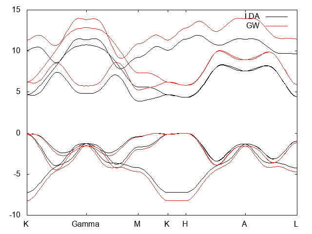
LDA and GW bands structure
![LDA and GW bands structure from Ref. [2]](/wiki/images/4/41/HBN_bands_lit.png)
LDA and GW bands structure from Ref. [2]

![LDA and GW bands structure from Ref. [2]](/wiki/index.php?title=File:HBN_bands_lit.png)
- As expected the effect of the GW correction is to open the gap.
- Comparing the obtained band structure with the one found in the literature by Arnaud and coworkers [2] we found a very nice qualitative agreement.
- Quantitatively we found a smaller gap: about 5.2 eV (indirect gap), 5.7 eV (direct gap) while in Ref.[2] is found 5.95 eV for the indirect gap and a minimum direct band gap of 6.47 eV. Other values are also reported in the literature depending on the used pseudopotentials, starting functional and type of self-consistency (see below).
- The present tutorial has been done with a small k point grid which is an important parameter to be checked, so convergence with respect the k point sampling has to be validated.
Step 4: Summary of the convergence parameters
We have calculated the band structure of hBN starting from a DFT calculation, here we summarize the main variable we have checked to achieve convergence:
EXXRLvcs# [XX] Exchange RL components
Number of G-vectors in the exchange. This number should be checked carefully. Generally a large number is needed as the QP energies show a slow convergence. The calcualtion of the exchange part is rather fast.
BndsRnXp#[Xp] Polarization function bands
Number of bands in the independent response function form which the dielectric matrix is calculated. Also this paramater has to be checked carefully,together with NGsBlkXp as the two variables are interconnected
NGsBlkXp# [Xp] Response block size
Number of G-vectors block in the dielectric constant. Also this paramater has to be checked carefully, to be checked together with BndsRnXp. A large number of bands and block can make the calculation very demanding.
LongDrXp# [Xp] [cc] Electric Field
Direction of the electric field for the calculation of the q=0 component of the dielectric constant e(q,w). In a bulk can be set to (1,1,1), attention must be paid for non 3D systems.
PPAPntXp# [Xp] Plasmon pole imaginary energy: this is the second frequency used to fit the Godby-Needs plasmon-pole model (PPM). If results depend consistently by changing this frequency, the PPM is not adequate for your calculation and it is need to gp beyond that, e.g. Real-axis.
GbndRnge# [GW] G[W] bands range
Number of bands used to expand the Green's function. This number is usually larger than the number of bands used to calculated the dielectricconstant. Single quasiparticle energies converge slowly with respect GbndRnge, energy difference behave better. You can use terminator technique to mitigate the slow dependence.
GDamping# [GW] G[W] damping
Small damping in the Green's function definition, the delta parameter. The final result shouuld not depend on that, usually set at 0.1 eV
dScStep# [GW]
Energy step to evaluate Z factors
DysSolver# [GW] Dyson Equation solver ("n","s","g")
Parameters related to the solution of the Dyson equation, "n" Newton linearization, 's' non linear secant method
GTermKind[GW] GW terminator
Terminator for the self-energy[1] . We have seen how this spped up the convergence with respect empty bands.
QPkrange# [GW] QP generalized Kpoint/Band indices
K-points and band range where you want to calculate the GW correction. The syntax is first kpoint | last kpoint | first band | last band
Step 5: Eigenvalue only self-consistent evGW0 and evGW
We moved self-consistent GW in a new separate tutorial: Self-consistent GW on eigenvalues only
Step 6: A better integration of the q=0 point
The integration of the q=0 of the Coulomb potential is problematic because the 1/q diverges. Usually in Yambo this integration is performed analytically in a small sphere around q=0.

however in this way the code lost part of the integral out of the circle. This usually is not problematic because for a large number of q and k point the missing term goes to zero. However in system that requires few k-points or even only the gamma one, it is possible to perform a better integration of this term by adding the flag -r to generate the input
HF_and_locXC                 # [R XX] Hartree-Fock Self-energy and Vxc
ppa                          # [R Xp] Plasmon Pole Approximation
gw0                          # [R GW] GoWo Quasiparticle energy levels
rim_cut                      # [R] Coulomb potential
em1d                         # [R Xd] Dynamical Inverse Dielectric Matrix
RandQpts= 3000000                     # [RIM] Number of random q-points in the BZ
RandGvec=  1            RL      # [RIM] Coulomb interaction RS components
#QpgFull                       # [F RIM] Coulomb interaction: Full matrix
EXXRLvcs = 40.000     mRy    # [XX] Exchange RL components
VXCRLvcs = 3187        RL      # [XC] XCpotential RL components
Chimod= "Hartree"                   # [X] IP/Hartree/ALDA/LRC/BSfxc
% BndsRnXp
  1 | 10 |                 # [Xp] Polarization function bands
%
NGsBlkXp= 1000          mRy    # [Xp] Response block size
% LongDrXp
 1.000000 | 1.000000 | 1.000000 |        # [Xp] [cc] Electric Field
%
PPAPntXp = 27.21138     eV    # [Xp] PPA imaginary energy
%GbndRnge
  1 | 40 |                 # [GW] G[W] bands range
%
GDamping=  0.10000     eV    # [GW] G[W] damping
dScStep=  0.10000      eV    # [GW] Energy step to evaluate Z factors
DysSolver= "n"               # [GW] Dyson Equation solver ("n","s","g")
%QPkrange        # [GW] QP generalized Kpoint/Band indices
 7|  7|  8|  9|
%
in this input RandGvec is the component of the Coulomb potential we want integrate numerically,
in this case only the first one G=G'=0, and RandQpts is the number of random points
used to perform the integral by Monte Carlo.
If you turn one this integration you will get a slightly different band gap, but in the limit of large k points the final results will be the same of the standard method.
However this correction is important for systems that converge with few k-points or with gamma only.
Step 7: Taking into account the material anisotropy
Hexagonal Boron Nitride is an anisotropic material. This means that the contribution from the screening at q points near the q=0 term is very different, depending on the direction along which q=0 is approached. Indeed the response function is non-analytical around q=0. In an exact calculation, the q=0 term (which is computed via a limiting procedure along a specific direction) has zero weight and the integral over q is correctly represented by all other q-points. In real numerical calculations, however, the q-points grid is finite and the q=0 term has a finite weight. It is used to represent the value of the screening in the region around q=0. Since it can be computed doing the limiting procedure in different directions, the question is: along which direction should one calculate the dielectric constant that enters in the GW scheme?
If you run again this tutorial changing the direction of the q=0 point in GW calculation,
the variable LongDrXp, you will realize that the there gap correction changes.
In Yambo, there are two procedures to take into account this anisotropy of the dielectric tensor.
Scheme a, based on a Random Integration Method (available from Yambo 4.6)
First of all, you need to calculate the dielectric constant in the three cartesian directions with the command yambo -o c -k hartree
optics                         # [R] Linear Response optical properties
kernel                         # [R] Kernel
chi                            # [R][CHI] Dyson equation for Chi.
dipoles                        # [R] Oscillator strenghts (or dipoles)
Chimod= "HARTREE"              # [X] IP/Hartree/ALDA/LRC/PF/BSfxc
NGsBlkXd= 3000        mRy      # [Xd] Response block size
% QpntsRXd
  1 | 1 |                       # [Xd] Transferred momenta
%
% BndsRnXd
   1 | 100 |                   # [Xd] Polarization function bands
%
% EnRngeXd
  0.00000 | 10.00000 | eV      # [Xd] Energy range
%
% DmRngeXd
  0.10000 |  0.10000 | eV      # [Xd] Damping range
%
ETStpsXd= 1                    # [Xd] Total Energy steps
% LongDrXd
 1.000000 | 0.000000 | 0.000000 |        # [Xd] [cc] Electric Field
%
From the result in the output file o.eps_q1_inv_rpa_dyson you can calculate the zero component of inverse dielectric matrix, in this case 1.0/5.044076 = 0.198252.
Repeat this calculation with the field in the other two directions y and z. The y-direction is equal to x, while in z direction the zero component of the inverse dielectric matrix is 1.0/2.872451 = 0.348134.
Now generate a new input file for the GW, with the command yambo -g n -p p -r -V RL
HF_and_locXC                 # [R XX] Hartree-Fock Self-energy and Vxc
ppa                          # [R Xp] Plasmon Pole Approximation
gw0                          # [R GW] GoWo Quasiparticle energy levels
rim_cut                      # [R] Coulomb potential
em1d                         # [R Xd] Dynamical Inverse Dielectric Matrix
RandQpts=3000000                     # [RIM] Number of random q-points in the BZ
RandGvec= 1            RL      # [RIM] Coulomb interaction RS components
#QpgFull                       # [F RIM] Coulomb interaction: Full matrix
% Em1Anys
  0.198252     | 0.198252     |   0.348134   |        # [RIM] X Y Z Static Inverse dielectric matrix
%
IDEm1Ref= 1
EXXRLvcs = 40.000     mRy    # [XX] Exchange RL components
VXCRLvcs = 3187        RL      # [XC] XCpotential RL components
Chimod= "Hartree"                   # [X] IP/Hartree/ALDA/LRC/BSfxc
% BndsRnXp
  1 | 10 |                 # [Xp] Polarization function bands
%
NGsBlkXp= 1000          mRy    # [Xp] Response block size
% LongDrXp
 1.000000 | 0.000000 | 0.000000 |        # [Xp] [cc] Electric Field
%
PPAPntXp = 27.21138     eV    # [Xp] PPA imaginary energy
%GbndRnge
  1 | 40 |                 # [GW] G[W] bands range
%
GDamping=  0.10000     eV    # [GW] G[W] damping
dScStep=  0.10000      eV    # [GW] Energy step to evaluate Z factors
DysSolver= "n"               # [GW] Dyson Equation solver ("n","s","g")
%QPkrange        # [GW] QP generalized Kpoint/Band indices
 7|  7|  8|  9|
%
run the calculations and you will find a correction of the gap intermediate between the one with the field in x and z directions.
Scheme b, based on averaging along the three directions (from Yambo 5.1)
This scheme computes the q=0 term three times, along three different directions, and then does an average. You just need to add in input the variable
OptDipAverage                      # [Xd] Average Xd along the non-zero Electric Field directions
% LongDrXd
 1.0000 | 1.0000 | 1.0000 |        # [Xd] [cc] Electric Field
%
If you have a 2D material you may want to average in-plane only. In such case you just need
OptDipAverage
% LongDrXd
 1.0000 | 1.0000 | 0.0000 |        # [Xd] [cc] Electric Field
%
Step 8: Exercise: Convergence with respect K points
As an exercise now you can check the convergence with respect the K point sampling:
- perform a new non-scf calculation with a bigger k point grid: 9x9x3 and 12x12x4 ...
- convert wave functions and electronic structure to Yambo databases in a different directory as explained in the DFT and p2y module,
- Initialize the Yambo databases,
- Redo the steps explained in this section (exchange self energy, plasmon pole GW, band structure interpolation)
- The PPA-GW calculation using 12x12x4 grid depending on your machine can take several minutes in serial mode. You can think to perform the exercise after having learned some basic on the parallelization strategy.
| Prev: Tutorials Home | Now: Tutorials Home --> GW | Next: If you did everything, choose another tutorial in the menu |