Calculating optical spectra including excitonic effects: a step-by-step guide

WORK IN PROGRESS - by Myrta Grüning

This tutorial guides you through the workflow of a calculation of the optical spectrum of a given material by solving the Bethe-Salpeter equation. Specifically we will use bulk h-BN as an example.

Before starting, you need to obtain the tarballs for hBN. See instructions on the main tutorials page.

Background

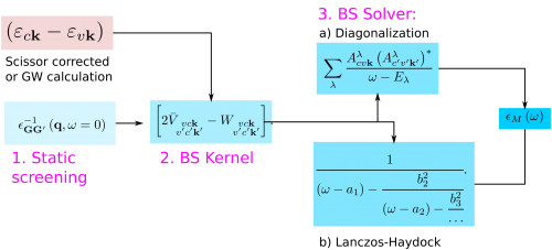
The target quantity in a Bethe-Salpeter calculation is the macroscopic dielectric matrix ε_M. The following quantities/steps are needed to obtain ε_M:

The optical absorption spectrum corresponds to Imε_M(ω).

Calculating the effective two-particle Hamiltonian

This first part calculates and stores the two-particle Hamiltonian matrix elements:

where vck indicates the pair of quasiparticle states vk and ck. The first term on the RHS is the quasiparticle energy differences (diagonal only). The second term is the kernel which is the sum of the electron-hole exchange part V (which stems from the Hartree potential) and the electron-hole attraction part W (which stems from the screened exchange potential). The kernel both shifts (diagonal contributions) and couples (off-diagonal contributions) the quasiparticle energy differences.

We start the calculation by running the initialization step (i.e. invoke yambo from the command line in the directory containing the relevant SAVE directory).

Step1: Calculation of the static dielectric screening.

Next, to calculate the correlation part of the kernel W we need the static dielectric screening. This is a calculation of the linear response of the system analogous to the calculation of the RPA/IP dielectric function. One important difference is that here we consider the static dielectric function.

Start by generating the input by invoking yambo with the option "-b" from the command line:

$ yambo -b -F 01_3D_BSE_screening.in

The input opens in the standard editor. Similarly to the other linear response calculations the relevant input variables to be changed are:

% BndsRnXs
  1 | 40 |                 
%
 NGsBlkXs= 4 Ry

The first variable gives how many bands are included in the sum to calculate the static response function. The second is a cutoff for the dimension of the static dielectric matrix.

In the next tutorial you will see how to choose these two parameters. Another relevant input parameter to change is

% LongDrXs
 1.000 | 1.000| 1.000
%

so that the perturbing electric field has component in each direction.

Run the calculation by invoking yambo:

$ yambo -F 01_3D_BSE_screening.in -J 3D_BSE 

In the log (l_em1s) of the calculation you can see that after calculating the dipole matrix elements, for each q vector yambo calculates the IP response function and by inversion the RPA response function

<02s> Xo@q[1] |########################################| [100%] --(E) --(X)
<02s> X@q[1] |########################################| [100%] --(E) --(X)

In the report, r_em1s, the details of the calculations are reported under the 5th section

[05] Static Dielectric Matrix
=============================

This calculation does not produce any human readable output, but both the dipole matrix elements and the static screening dielectric function are saved in a database in the 3D_BSE directory:

3D_BSE/ndb.dip_iR_and_P
3D_BSE/ndb.em1s

which are needed and read by the following yambo runlevels.

Step2: Calculation of matrix elements of the BSE kernel

You have now all ingredients to calculate the kernel

(and thus the two-particle Hamiltonian matrix elements).

Start by generating the input by invoking yambo with the option "-o b -k bse -V qp" from the command line:

$ yambo -o b -k bse -V qp -F 02_3D_BSE_kernel.in

The input opens in the standard editor. The relevant input parameters to be changed are

BSENGexx = 30 Ry
BSENGBlk = 4 Ry
% BSEBands
 6 | 10 |       
%

The first two are the cutoff for the summations on the reciprocal lattice vectors which appear in the expressions for V (BSENGexx) and W (BSENGBlk) here above.

The third parameter gives the range of quasiparticle states (their band index) that define the basis of quasiparticle pairs that we need to describe the excitons (in the energy range of interest). For example since we have 8 occupied bands, here we consider the pairs of bands: 6-9, 6-10, 7-9, 7-10, 8-9, 8-10 (those are 6 pairs of bands = 2 valence times 3 conduction bands).

For each of those pairs we then consider all k points in the Brillouin zone available from the DFT calculations. Since we have a 6 x 6 x 2 grid, this amounts to 72 k points in the Brillouin zone.

Then finally we are using a basis of 6 x 72 = 432 vck pairs to represent the excitons of the system.

The values for these 3 parameters are chosen from convergence studies, as discussed in the next tutorial.

Another parameter to modify is

% KfnQP_E 
 1.440000 | 1.000000 | 1.000000 |
%

This gives the quasiparticle corrections to the Kohn-Sham eigenvalues and is deduced either from experiment or previous GW calculations. The corrections consist in a shift (first value) of the conduction bands in eV and renormalization of the conduction and valence bandwidths (second and third value). Alternatively we can directly input corrections calculated from a previous GW calculation as we will learn later in this tutorial.

Run the calculation by invoking yambo in the command line:

$ yambo -F 02_3D_BSE_kernel.in -J 3D_BSE 

In the log (either in standard output or in l_optics_bse_bsk), after various setup/loading, the kernel is calculated:

<01s> [05.04.03] Kernel loop
<02s> Kernel |########################################| [100%] --(E) --(X)

In the report r_optics_bse_bsk the information relative to this runlevel are reported under the section:

[05] Response Functions in Transition space
===========================================

Take some time to inspect the log and the report. For example try to find where the input parameters are reported, the dimension of the 2-particle hamiltonian and if these match your expectations.

This run does not produce any human readable output. The kernel is stored in a database in the 3D_BSE directory

3D_BSE/ndb.BS_Q1

Obtaining the optical spectrum from the two-particle Hamiltonian

The macroscopic dielectric function (from which the absorption and EEL spectra can be computed) is obtained from the eigenvalues E_λ (excitonic energies) and eigenvectors A^λ_cvk (exciton composition in terms of electron-hole pairs) of the two-particle Hamiltonian:

To get the two-particle Hamiltonian eigensolutions you can either

(1) diagonalize the full Hamiltonian (diagonalization solver)

(2) use the subspace iterative Lanczos algorithm and by-pass diagonalization with the Haydock approach (Lanczos-Haydock solver)

Both approaches are detailed here below.

Diagonalization solver

Invoke yambo with the "-y d" option in the command line:

$ yambo -y d -F 03_3D_BSE_diago_solver.in

The input is open in the editor. The input variable to be changed are

% BEnRange
  2.00000 | 8.00000 | eV    
%
BEnSteps= 200      

which define 200 evenly spaced points between 2 and 8 eV at which the spectrum is calculated (ω in the equation for the macroscopic dielectric function),

% BDmRange
  0.10000 |  0.10000 | eV    
%

which defines the spectral broadening (Lorentzian model),

% BLongDir
 1.000000 | 1.000000 | 0.000000 | 
%

which defines the direction of the perturbing electric field (in this case the in-plane direction).

Run yambo:

$ yambo -F 03_3D_BSE_diago_solver.in -J 3D_BSE  

In the log (either in standard output or in l-3d_BSE_optics_bse_bsk_bss), after various setup/loading, the BSE is diagonalized using the linked linear algebra libraries:

<01s> [06] BSE solver(s)
<01s> [LA] SERIAL linear algebra
<01s> [06.01] Diagonalization solver
<01s> BSK diagonalize |########################################| [100%] --(E) --(X)
<01s> EPS   residuals |########################################| [100%] --(E) --(X)
<01s> BSK     epsilon |########################################| [100%] --(E) --(X)

The report r-3d_BSE_optics_bse_bsk_bss contains information relative to this runlevel in section 6:

[06] BSE solver(s)
==================

Take some time to inspect the log and the report to check the consistency with the input variables. This run produces a new database in the 3D_BSE directory

3D_BSE/ndb.BS_diago_Q01

So if you need the spectrum on a different energy range, direction, with a different broadening or on more points the diagonalization is not repeated, just the spectrum is recalculated.

This run produces as well human readable files (o-*). Specifically o-3D_BSE.eps_q1_diago_bse contains the real and imaginary part of the macroscopic dielectric function

$ less o-3D_BSE.eps_q1_diago_bse 
...
#
#  E/ev[1]    EPS-Im[2]  EPS-Re[3]  EPSo-Im[4] EPSo-Re[5]
#
  2.00000    0.16162    5.83681    0.04959    4.14127
  2.03015    0.16787    5.88612    0.05090    4.15638
...

which is in the format

Energy in eV | Imaginary part BSE | Real part BSE |Imaginary part IPA | Real part IPA |  

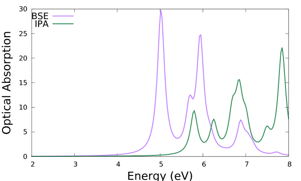
where real and imaginary parts refer to the macroscopic dielectric function. The imaginary part corresponds to the optical absorption. The latter (column 2) can be plotted versus the photon energy (column 1) and compared with the independent particle approximation (IPA, column 4), e.g.:

$ gnuplot
...
plot 'o-3D_BSE.eps_q1_diago_bse' u 1:2 w l t 'BSE', 'o-3D_BSE.eps_q1_diago_bse' u 1:4 w l  t 'IPA'

The addition of the kernel has the effect to red-shift the spectrum onset and to redistribute the oscillator strengths. Note that the convergence with respect to k-points smooths out the low energy peaks in the IPA (which are an artifact of poor convergence with k-points producing an artificial confinement) to give the shoulder corresponding to the van Hove singularity in the band structure. On the other hand the low energy peak in the BSE is genuine and it is the signature of a bound exciton.

Lanczos-Haydock solver

You can avoid the full matrix diagonalization (which rapidly become expensive as it scales as N³) by using the Lanczos-Haydock solver mentioned above. While for small matrices these two methods have similar computational cost, for matrices of the size 10000 by 10000 and larger, the Haydock solver is remarkably faster. The drawback is that excitonic functions cannot be calculated. Within the Lanczos-Haydock approach the macroscopic dielectric function is rewritten as continued fraction

where a 's and b 's result from the Lanczos iterative algorithm.

To use the Lanczos-Haydock solver invoke yambo with "-y h" option in the command line:

$ yambo -y h -F 03_3D_BSE_haydock_solver.in

Beside the same input parameters defined for the diagonalization solver, the parameter

BSHayTrs= -0.02000          

defines the threshold accuracy for the Lanczos-Haydock iterative process: the calculation stops when the difference between two consecutive calculated spectra is smaller than the absolute value of the threshold. The minus sign indicates that the average difference over the specified energy range is considered (i.e. that means that cancellations of error may occur) as opposed to the maximum absolute difference over the specified energy range (plus sign). For the moment we leave this variable unchanged. This parameter ultimately determines the terms are included in the continued fraction here above. Later we explore how this variable influences the final result.

Invoke yambo to run the calculation:

$ yambo -F 03_3D_BSE_haydock_solver.in -J "3D_BSE-low,3D_BSE"  

This outputs the following log:

...
<01s> [06] BSE solver(s)
<01s> [06.01] Haydock solver
<01s> [Haydock] Iteration 1
<03s> [Haydock] Iteration 21 Accuracy :  0.01647| -0.02000
...

The Lanczos-Haydock iterative procedure converged to the desired accuracy in 21 iterations.

This runs only produces human readable files. That means that if you changes the input parameters (such as the broadening or the energy range) the Lanczos-Haydock procedure has to be repeated. Among the human readable files, o-3D_BSE-low.eps_q1_haydock_bse contains the real and imaginary part of the macroscopic dielectric function:

$ less o-3D_BSE-low.eps_q1_haydock_bse
...
#
#  E/ev[1]    EPS-Im[2]  EPS-Re[3]  EPSo-Im[4] EPSo-Re[5] EPS`-Im[6] EPS`-Re[7]
#
   2.00000    0.16089    5.81293    0.04945    4.12727    0.16089    5.81293
   2.03015    0.16711    5.86203    0.05076    4.14234    0.16711    5.86203
...

This file has a slightly different data structure with respect to the diagonalization solver:

Energy in eV | Imaginary part BSE | Real part BSE |Imaginary part IPA | Real part IPA |Imaginary part BSE (it-1) | Real part BSE (it-1)|

We can plot the second and sixth columns and compare with the result from diagonalization:

$gnuplot
...
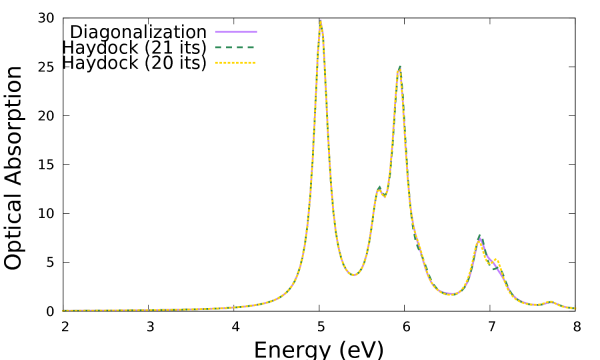
 plot 'o-3D_BSE.eps_q1_diago_bse' u 1:2 w l t 'Diagonalization', 'o-3D_BSE-low.eps_q1_haydock_bse' u 1:2 w l t 'Haydock (27 its)', 'o-3D_BSE-low.eps_q1_haydock_bse' u 1:6 w l t 'Haydock (26 its)'

Except for the peak at higher energy, the results on this scale are identical to those obtained via the diagonalization solver. By comparing the results for the Lanczos-Haydock solver at 27 and 26 iterations, it is clear that the difference with the diagonalization results can be eliminated by lowering the threshold for the iterative process.

Repeat now the calculation by changing the input variable:

BSHayTrs= 0.02000          

which enforces a stricter condition on the convergence of the iterative process (see above)

Running yambo:

$ yambo -F 03_3D_BSE_haydock_solver.in -J "3D_BSE-high,3D_BSE"  

outputs the following log

...
<01s> [06] BSE solver(s)
<01s> [06.01] Haydock solver
<01s> [Haydock] Iteration 1
<06s> [Haydock] Iteration 45 Accuracy :   0.0098|  0.02000
...

Now 45 iterations, rather than 21, were needed to reach the desired accuracy. By plotting these results:

$ gnuplot
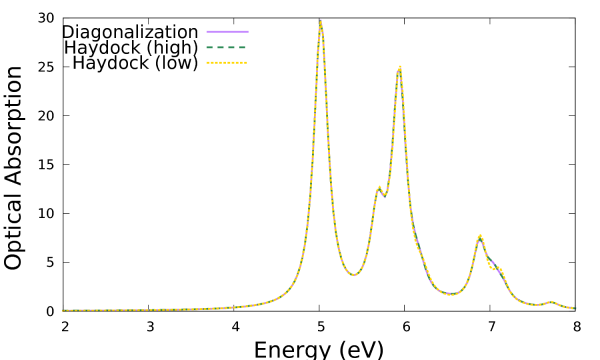
plot 'o-3D_BSE.eps_q1_diago_bse' u 1:2 w l ls 1 t 'Diagonalization', 'o-3D_BSE-high.eps_q1_haydock_bse' u 1:2 w l ls 2 t 'Haydock (high)', 'o-3D_BSE-low.eps_q1_haydock_bse' u 1:2 w l ls 3 t 'Haydock (low)'

Which shows that the Lanczos-Haydock solver with the stricter convergence criterion and the diagonalization solver are identical on this scale.

Some more advanced options

Reading the QP corrections from a previous GW calculation

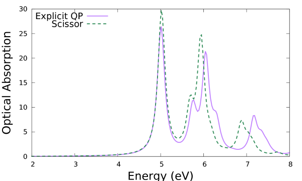
In the above calculation we have used a simple scissor operator to correct the Kohn-Sam DFT energies. In this part we see how we can instead take the corrections from a previous Yambo Gw calculation. We create and edit the input. This time instead of proceeding in three steps as before, we create one input performing all three steps:

$yambo -o b -k sex -y d -V qp -F Ins/05_3D_QP_BSE.in

We set all parameters as in the previous calculation, except for the part regarding the QP correction:

 KfnQPdb= "E < 3D_QP_BSE/ndb.QP"              # [EXTQP BSK BSS] Database
 KfnQP_N= 1                   # [EXTQP BSK BSS] Interpolation neighbours
 % KfnQP_E
  0.000000 | 1.000000 | 1.000000 |        # [EXTQP BSK BSS] E parameters  (c/v) eV|adim|adim
%

Instead of setting the values for the scissor, we give the path to a database (3D_QP_BSE/ndb.QP) which contains the QP corrections. This has been created by running a GW calculation as in the GW tutorial. Run Yambo:

$ yambo -F Ins/05_3D_QP_BSE.in -J "3D_QP_BSE,3D_BSE"

This produces the following log in the standard output. Note Section 4 (regarding external QP corrections to the kernel):

<01s> [04.01] External QP corrections (K)
<01s> [QP@K] E<3D_QP_BSE/ndb.QP[ PPA XG:39 Xb:1   40 Scb:1   40]
<01s> [QP] Kpts covered exactly  [o/o]: 100.0000

This tells you that the file was found, read correctly and that the k points found in the file matched the ones you are using for the current calculation (otherwise interpolation would be needed). It is crucial to check that the file has been read, since if not Yambo gives a warning but continues the calculation (with no QP corrections at all!). As in the previous calculation the final results of the calculation are the files with the spectral functions. Let's compare the results for the optical absorption spectrum with those obtained previously with a simple scissor:

$ gnuplot
...
plot 'o-3D_QP_BSE.eps_q1_diago_bse' u 1:2 w l t 'Explicit QP', 'o-3D_BSE.eps_q1_diago_bse' u 1:2 w l t 'Scissor' 

It is clear that this makes a difference in the peak distribution and intensity. Note that beside a simple shift you can renormalise as well the bandwidth of the valence and conduction bands in KfnQP_E (respectively the third and second value). You can try as an exercise to set up a new calculation using e.g. 1.440000 | 1.200000 | 0.900000 | for KfnQP_E.