Third Harmonic Generation (THG)
Third Harmonic Generation in bulk Silicon
In this tutorial we will calculate third harmonic generation (THG) in bulk Silicon.
Calculation of third harmonic generation proceeds in similar way to the SHG calculations.
DFT input can be found here (abinit or QuantumEspresso).
We import the wave-functions as explained in the Real time approach to non-linear response, then perform the setup using only 1000 plane waves.
Removing symmetries
We are interested in the [math]\displaystyle{ \chi^{(3)}_{1111} }[/math] therefore we consider an external field in direction [1, 0, 0] (equivalent to [x,0,0]).
We remove all the symmetries not compatible with the external field plus the time-reversal symmetry by doing ypp_nl (or ypp) -y:
fixsyms                      # [R] Reduce Symmetries
% Efield1
 1.00     | 0.00     | 0.00     |        # First external Electric Field
%
% Efield2
 0.00     | 0.00     | 0.00     |        # Additional external Electric Field
%
#RmAllSymm                   # Remove all symmetries
RmTimeRev                   # Remove Time Reversal
Real-time simulations
Then you go in the FixSymm folder, run again the setup (as explained in the Linear response using Dynamical Berry Phase) and then generate the input file with the command yambo_nl -u n -V qp -F input.in:
nloptics                      # [R NL] Non-linear optics
% NLBands
  1 | 7 |                   # [NL] Bands
%
NLstep=   0.0100       fs    # [NL] Real Time step length
NLtime=-1.000000       fs    # [NL] Simulation Time
NLintegrator= "CRANKNIC"     # [NL] Integrator ("EULEREXP/RK4/RK2EXP/HEUN/INVINT/CRANKNIC")
NLCorrelation= "IPA"         # [NL] Correlation ("IPA/HARTREE/TDDFT/LRC/JGM/HF/SEX")
NLLrcAlpha= 0.000000         # [NL] Long Range Correction
% NLEnRange
 0.200000 | 2.000000 |  eV    # [NL] Energy range
%
NLEnSteps=  6               # [NL] Energy steps
NLDamping= 0.200000    eV    # [NL] Damping
%Field1_Dir
  1.000000 | 0.000000 | 0.000000 |        # [RT Field1] Versor
Field1_kind= "SOFTSIN"         # [NL ExtF] Kind(SIN|SOFTSIN|RES|ANTIRES|GAUSS|DELTA|QSSIN)
Field1_Int= 0.1000E+8         kWLm2 # [NL ExtF] Intensity
 % GfnQP_E
 0.600000 | 1.000000 | 1.000000 |        # [EXTQP G] E parameters  (c/v) eV|adim|adim
 %
We calculate the [math]\displaystyle{ \chi^{(3)}_{1111} }[/math] only on 6 frequencies, but calculations can be extended to larger frequency range.
We introduce a scissor operator of 0.6 eV in such a way to reproduce the gap of bulk silicon. Notice that we increased the field intensity in such a way to improve the ratio between non-linear response and numerical noise.
Now that you have created the file input.in you can run the non-linear optics calculation with the command:
yambo_nl -F input.in
when the simulation will end, it will have produced the file SAVE/ndb.Nonlinear with all information on the simulation and the files SAVE/ndb.Nonlinear_fragment_x with the polarization and current for each laser frequency.
Analysis of the results
Results can be analyzed in the same way of the SHG, using the command ypp_nl -u:
nonlinear                    # [R] NonLinear Optics Post-Processing
Xorder=  5                   # Max order of the response functions
% TimeRange
 40.000000 | -1.00000 | fs    # Time-window where processing is done
%
ETStpsRt= 200                # Total Energy steps
% EnRngeRt
 0.00000 | 10.00000 | eV    # Energy range
%
DampMode= "NONE"             # Damping type ( NONE | LORENTZIAN | GAUSSIAN )
DampFactor=  0.10000   eV    # Damping parameter
This time we increase the de-phasing time to 40 fs in such a way to have a clean third-harmonic response.
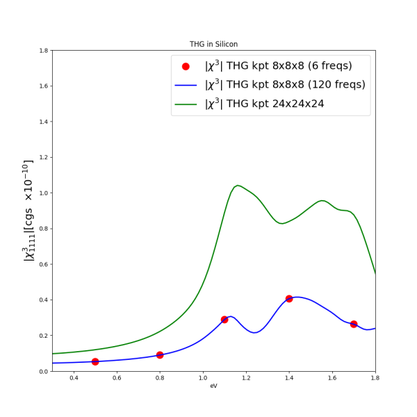
Hereafter we report the result with the 8x8x8 k-points sampling and the converged result with the 24x24x24 k-points sampling:
Plot data can be downloaded here.
Analysis of the results with YamboPy
This part works only with Yambo 5.3 or the last version available on Github: https://github.com/yambo-code/yambo
The previous analysis can be performed using YamboPy, see these other tutorials for more details (Real time approach to non-linear response#Analysis of the results using YamboPy)
From the folder of the calculations in python you use the script:
from yambopy import *
from yambopy.plot  import *
from yambopy.units import fs2aut

NLDB=YamboNLDB()

pol =NLDB.Polarization[0]
time=NLDB.IO_TIME_points

Harmonic_Analysis(NLDB,X_order=5,T_range=[40.0*fs2aut,-1.0])
it will produce files with the non-linear response o.YamboPY-X_probe_order_x equivalent to the ones produced by ypp_nl.
How to choose the external field direction for the different X3
In the X3abcd response you have four field directions. The three components b,c and d are determined by the external field and the four a
is the direction where you measure the response.
The external field in Yambo is set using the variable
%Field1_Dir
 1.000000 | 0.000000 | 0.000000 |        # [NL ExtF] Versor .
%
For example if you set in Yambo field direction as:
1.0 | 0.0 | 0.0 | ---> you calculate all components X3*xxx
0.0 | 1.0 | 0.0 | ---> you calculate all components X2*yyy
0.0 | 0.0 | 1.0 | ---> you calculate all components X2*zzz
the * correspond to the different direction in the response file o.YPP-X_probe_order_3.
In the o.YPP-X_probe_order_3 you have seven columns:
The first column is the energy omega,
the 2nd and 3rd columns are the imaginary and real part of X3x***
the 4th and 5th columns are the imaginary and real part of X3y***
the 6th and 7th columns are the imaginary and real part of X3z***
where the *** are the direction of the incoming field, see above.
Instead for an external field in Yambo in the direction
%Field1_Dir
 1.000000 | 1.000000 | 1.000000 |        # [NL ExtF] Versor .
%
you can get in output in the o.YPP-X_probe_order_3 file the components:
the 2nd and 3rd columns are the imaginary and real part of X3xxyz
the 4th and 5th columns are the imaginary and real part of X3yxyz
the 6th and 7th columns are the imaginary and real part of X3zxyz
Other terms of the X3 tensor can be obtained combining the different columns of the o.YPP-X_probe_order_3 file and using external fields along linear combination of the Cartesian axes.
Nota bene: if you change the direction of the external field you have to remove the corresponding symmetries as explained in the tutorial on Prerequisites for Real Time propagation with Yambo#Reduce symmetries real-time linear response tutorial.
