Linear response using Dynamical Berry Phase
The tutorial on linear response from real-time Schödinger equation is divided in 8 steps:
DFT calculations
In Yambo all quantities are written in a basis of the Kohn-Sham(KS) eigenvalues and eigenvectors. In order to generate this basis we use a DFT code in plane wave as Abinit or QuantumEspresso(QE).
In this example we will consider a single later of hexagonal boron nitrite (hBN), the input files available here (QE_inputs or ABINIT_inputs). The first input file is a self-consistent(SCF) calculation that is used to generate the density of the system. The second input file is a non-self consistent(NSCF) calculation to diagonalize the KS Hamiltonian, that depends from the density of the first run, on for a given number of bands and k-points. Notice that parameters in the NSCF calculation determine the number of k-points and the maximum number of bands that can be used in Lumen. Run these calculation with the command:
for QuantumEspresso:
pw.x -inp BNsheet.scf.in  > output_scf
pw.x -inp BNsheet.nscf.in > output_nscf
for Abinit:
abinit < hBN.files > output_hBN
Notice that in the NSCF file of QuantumEspresso we use the flag force_symmorphic=.true. to exclude the non-symmorphic symmetries that are not supported by Yambo, in Abinit the same option is activated by the flag symmorphi 0.
Import the wave-functions
If you used QuantumEspresso go in the folder bn.save, in the ABINIT case all file are already in the main folder. Then import the wave-function with the command
for QuantumEspresso:
p2y
for Abinit:
a2y -F hbn_out_DS2_KSS
Setup
Generate the setup input file with the command yambo_nl -i -V RL -F setup.in, then run yambo_nl -F setup.in.
You can reduce the number of G-vectors in the setup in such a way to speed up calculations. I advise to reduce G-vector to 1000 (about 50% the initial ones).
Reduce symmetries
Since in real-time simulation we introduce a finite electric field in the Hamiltonian, the number of the symmetries of the original system is reduced due to the presence of this field. Using the tool ypp -y to generate the input file:
fixsyms                      # [R] Reduce Symmetries
% Efield1
0.00     | 1.00     | 0.00     |        # First external Electric Field
%
% Efield2
 0.00     | 0.00     | 0.00     |        # Additional external Electric Field
%
#RmAllSymm                   # Remove all symmetries
RmTimeRev                   # Remove Time Reversal
Set the external field in the y direction and uncomment the Time Reversal flag, as shown in red above. Run ypp and it will create a new folder called FixSymm with the reduced symmetries wave-functions.
Setup again
Go in the FixSymm directory and run the setup again yambo_nl -F ../setup.in. Now everything is ready for the real-time simulations!
Real-time dynamics
In order to calculate linear-response in real-time we will perturb the system with a delta function in time external field. Use the command yambo_nl -u p -F input_lr.in to generate the input:
nlinear                      # [R NL] Non-linear optics
NL_Threads= 1                # [OPENMP/NL] Number of threads for nl-optics
% NLBands
  3 |  6 |                   # [NL] Bands
%
NLstep=   0.0100       fs    # [NL] Real Time step length
NLtime=55.000000      fs    # [NL] Simulation Time
NLintegrator= "INVINT"       # [NL] Integrator ("EULEREXP/RK4/RK2EXP/HEUN/INVINT/CRANKNIC")
NLCorrelation= "IPA"         # [NL] Correlation ("IPA/HARTREE/TDDFT/LRC/JGM/SEX/HF")
NLLrcAlpha= 0.000000         # [NL] Long Range Correction
NLDamping=  0.000000   eV    # [NL] Damping
RADLifeTime=-1.000000      fs    # [RT] Radiative life-time (if negative Yambo sets it equal to Phase_LifeTime in NL)
#EvalCurrent                   # [NL] Evaluate the current
#FrPolPerdic                   # [DIP] Force periodicity of polarization respect to the external field
% Field1_Freq
 0.100000 | 0.100000 |         eV    # [RT Field1] Frequency
%
Field1_NFreqs= 1                 # [RT Field1] Frequency
Field1_Int=  1000.00       kWLm2 # [RT Field1] Intensity
Field1_Width= 0.000000     fs    # [RT Field1] Width
Field1_kind=   "DELTA"           # [RT Field1] Kind(SIN|COS|RES|ANTIRES|GAUSS|DELTA|QSSIN)
Field1_pol= "linear"             # [RT Field1] Pol(linear|circular)
% Field1_Dir
   0.000000 | 1.000000 | 0.000000 |        # [RT Field1] Versor
%
Field1_Tstart= 0.010000    fs    # [RT Field1] Initial Time
The standard input of Lumen is thought for non-linear response so we have to change some parameters in order to calculate the linear response. Set the field direction along y, the field type to DELTA, the length of the simulation to 55 fs, number of bands from 3 to 6 dephasing to zero and the number of energy steps to one, as shown above in red.
We set the verbosity to "high" in such a way to print real-time output files.
We set the differential equation integrator to INVINT that is faster bul less accurate than the default(see PRB 88, 235113). This integrator is ok in case of independent partcicles but I advise you to use CRANKNIC integrator when correlation effects are present. Now run yambo_nl -F input_lr.in
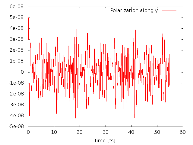
The code will produce different files: o.polarization_F1 that contains the polarization, o.external_potential_F1 the external field we used, and finally r_optics_nloptics a report with all information about the simulation. If you plot the third column of o.polarization_F1 versus the first one (time variable) you will get the time-dependent polarization along the y direction:
Analyze the results
Now we can use ypp_nl -u to analyze the results:
nonlinear                    # [R] NonLinear Optics Post-Processing
Xorder= 1                    # Max order of the response functions
% TimeRange
-1.000000 |-1.000000 | fs    # Time-window where processing is done
%
ETStpsRt= 200                # Total Energy steps
% EnRngeRt
  0.00000 | 10.00000 | eV    # Energy range
%
DampMode= "LORENTZIAN"             # Damping type ( NONE | LORENTZIAN | GAUSSIAN )
DampFactor=  0.10000   eV    # Damping parameter
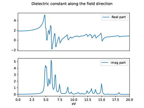
where we set a Lorentzian smearing corresponding to 0.1 eV. Notice that due to the finite time of our simulation a smearing is always necessary to Fourier transform the result. Then we run ypp_nl and obtain the following files: the dielectric constant along the field direction o.YPP-eps_along_E, the EELS along the same direction o.YPP-eels_along_E, and the damped polarization o.YPP-damped_polarization.
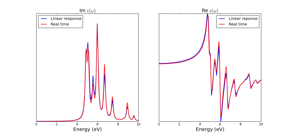
Now we can plot the dielectric constant and compare it with linear response:
The input for the linear response can be downloaded here. Notice that in a real-time simulation we obtain directly the [math]\displaystyle{ \chi(\omega) = \frac{P(\omega)}{E(\omega)} }[/math] that is related to the dielectric constant from the relation [math]\displaystyle{ \epsilon(\omega) = 1 + 4 \pi \chi(\omega) }[/math]
Analysis of the results using YamboPy
This part works only with Yambo 5.3 or the last version available on Github: https://github.com/yambo-code/yambo
Starting from Yambo 5.3 the analysis of real-time simulation can performed using YamboPy code.
Here we suppose that you already installed it otherwise you can follow this webpage Setting up YamboPy.
In order to analyze the real-time results, go in the folder where you ran the simulation, and in the python shell type:
import numpy as np
from yambopy import *
from yambopy.plot  import *

NLDB=YamboNLDB()

pol =NLDB.Polarization[0]
time=NLDB.IO_TIME_points
t_initial=NLDB.Efield[0]["initial_time"]
in this way you read all the Non-linear databases. If your runs are in a different folder then the 'SAVE' one you can specify it using the command:
NLDB=YamboNLDB(calc='MYJOB')
now in the array pol you have all the polarization for all laser frequencies in the three Cartesian directions, while the variable time contains all the time series of your simulation, and t_intital is the time when the external field is turned on.
We can now apply a damping function to the polarization before Fourier transform it by doing:
pol_damped=np.empty_like(pol)
for i_d in range(3):
   pol_damped[i_d,:]=damp_it(pol[i_d,:],time,t_initial,damp_type='LORENTZIAN',damp_factor=0.1/ha2ev)
now we can plot the damped polarization with the command
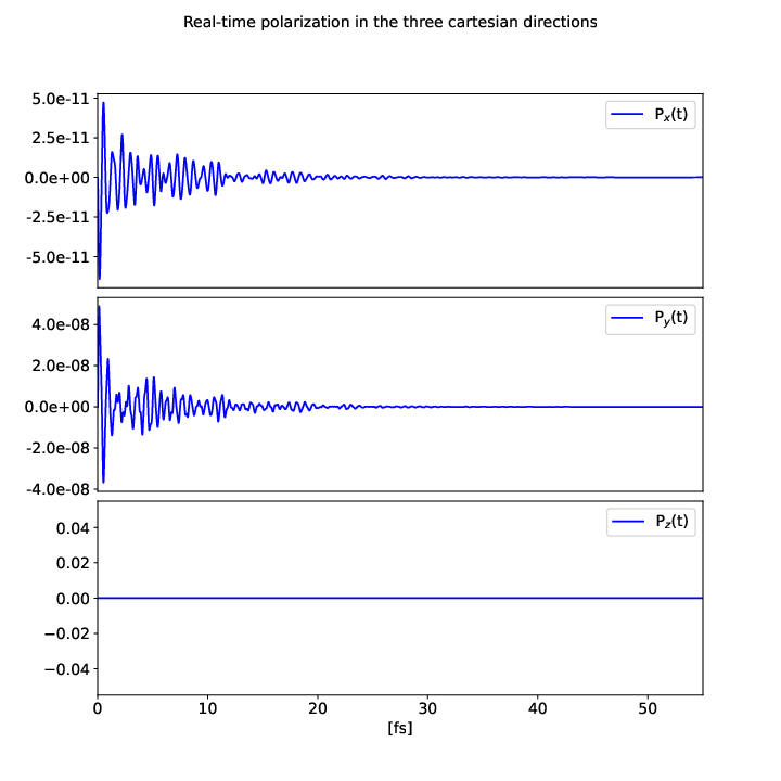
Plot_Pol_or_Curr(time=time, pol=pol_damped, xlim=[0,55], save_file='polarization.pdf')
you will get the damped polarization in the three Cartesian directions:
Now we can Fourier transform it to get the dielectric constant as explained in the previous section:
Linear_Response(time=time,pol=pol_damped,efield=NLDB.Efield[0],plot=False,plot_file='eps.pdf')
here the result:
