SOC
Effect of spin-orbit interaction
Introduction
The scope of this tutorial is to calculate the G0W0 corrections to the DFT-LDA band-structure and the BSE optical spectrum for a bulk semiconducting material, gallium antimonide (GaSb) [1][2][3][4]. We will compare the results with and without the spin-orbit interaction.

Zincblende crystalline structure. Two atoms per cell, Ga and Sb (8 electrons). Lattice constant 11.38 [a.u.]

Ground state: plane waves cutoff 18 Ry Large spin-orbit splitting of highest occupied bands: ~ 0.7eV
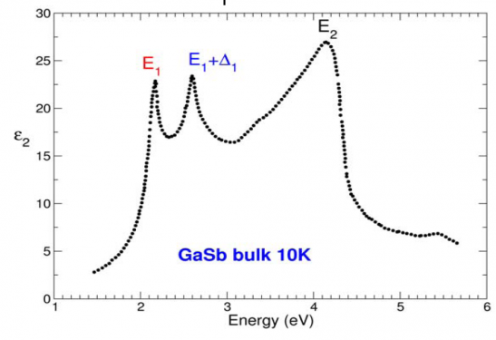
Large spin-orbit splitting of the E1 optical peak (E1, E1+D1) visible in the experimental optical spectrum
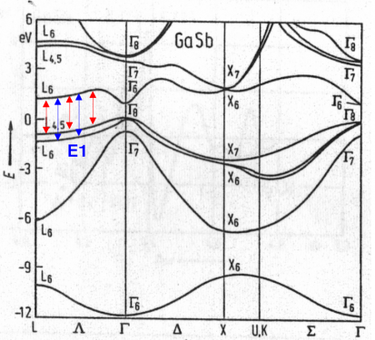
Origin in k-space of the E1 peak


DFT band structure
For this tutorial we provide two state (GS) databases (DBs), one contains the GS-DBs with the effect of SOC included and one without. The idea is to repeat the same calculation for both database and compare the results and the performances of the code. As in other tutorials you can find the folder containing the input files for the pwscf code (Pwscf, in case you prefer to generate the GS-DBs by yourself) and the folder containing the GS-DBs, the reference input files and the reference output files for the yambo code (YAMBO). Instead of continuously jumping back and forth from the Without_SOC to the With_SOC folder we advice to open two terminals and keep one for the without SOC case and another for the with SOC case.
Let's have a look to the content of the folders. For example we can enter in the Solid_GaSb/With_SOC/ folder
$ cd Solid_GaSb/With_SOC/
$ ls Pwscf YAMBO
$ cd YAMBO
$ ls 4x4x4_shifted+GAMMA
6x6x6_shifted  10x10x10_shifted 14x14x14_shifted   Inputs  Reference_Outputs
Inside the YAMBO folder there are indeed four folders corresponding to four differet k-points meshes. In this tutorial we will use the 4x4x4_shifted+GAMMA folder for the computation of the QP corrections within the GoWo approximation. It is a kpts grid obtained as the sum of a 4x4x4 k-points grid centered in Gamma and a 4x4x4 grid shifted. Instead for the computation of the optical properties we will use the 6x6x6_shifted folder. It is a 6x6x6 k-points grid shifted from Gamma. The other two folders, 10x10x10_shifted and 14x14x14_shifted can be used to do a minimum convergence of the optical properties against the number of k-points (pay attention that the BSE calculations with bigger grids will be very memory and time demanding!).
The first part of the tutorial is on the computation of the QP corrections. So let's enter the 4x4x4_shifted+GAMMA grid and, as seen in other tutorials run the Initialization:
$ cd 4x4x4_shifted+GAMMA/
$ yambo -J 01_init
Now compare the result of the two setup runs.
With_SOC case:
[02.05] Energies [ev] & Occupations
  ===================================

  Fermi Level        [ev]:  5.046557
  VBM / CBm          [ev]:   0.00000   0.06025
  Electronic Temp. [ev K]:  0.00      0.00
  Bosonic    Temp. [ev K]:  0.00      0.00
  El. density      [cm-3]: 0.146E+24
  States summary         : Full        Metallic    Empty
                           0001-0008               0009-0200
  Indirect Gaps      [ev]:  0.06025   3.57546
Without_SOC case:
[02.05] Energies [ev] & Occupations
  ===================================

  Fermi Level        [ev]:  4.777401
  VBM / CBm          [ev]:  0.000000  0.332282
  Electronic Temp. [ev K]:  0.00      0.00
  Bosonic    Temp. [ev K]:  0.00      0.00
  El. density      [cm-3]: 0.146E+24
  States summary         : Full        Metallic    Empty
                           0001-0004               0005-0100
  Indirect Gaps      [ev]: 0.332282  3.620628
  Direct Gaps        [ev]: 0.332282  7.137342
A clear shrink of the DFT-LDA gap due to spin-orbit occurs. Note that, having 8 electrons in the fundamental cell, due to the spinorial nature of the wavefunction, with SOC we have 8 occupied bands, while only 4 without. Here a picture of the DFT band structure for the two cases.

Effect of spin-orbit interaction on the band structure of GaSb
Now we will perform a G0W0 calculation to correct the DFT-LDA bandstructure. We assume that you are already familiar with the concept of screening needed to build up the GW self-energy and thus the QP corrections. Create a local folder My_inputs and generate the input for a G0W0 calculation within the plasmon-pole approximation using the following command:
$ cd 4x4x4_shifted+GAMMA
$ mkdir My_inputs
$ yambo -p p -g n -V RL -F My_inputs/02_GW.in
However we also provide an input file with suggested parameters for this calculations inside the folder Solid_GaSb/Without_SOC/Yambo/Inputs. Remember: these parameters are system dependent and should be converged as you can see other GW tutorials (e.g. GW or GW convergence). Here we provide reasonable (but not fully converged) parameters to have a low computational cost but yet qualitatively meaningful results.
The plane-waves cutoff for the wavefunctions and exchange part of the self-energy are set to 10 Ry.
FFTGvecs =  10 Ry   # [FFT] Plane-waves
EXXRLvcs=   10 Ry   # [XX] Exchange RL components
while we will use 40 bands, a plane-wave cut-off of 1 Ry, and a plasmon-pole energy of 20 eV to build up the screening matrix
NGsBlkXp=    1 Ry  # [Xp] Response block size
PPAPntXp= 20.  eV  # [Xp] PPA imaginary energy
% BndsRnXp
1 | 40 |        # [Xp] Polarization function bands
%
% LongDrXp
1.000000 | 1.000000 | 1.000000 |        # [Xp] [cc] Electric Field
%
The number of bands in the green function G to build up the GW self-energy is also 40
% GbndRnge
1 | 40 |                 # [GW] G[W] bands range
%
with those parameters we will compute the correction only in the last 2 points of our grid, 28 and 29 and for the states from 3 to 6, setting the input variable
%QPkrange
28 | 29 |   3 | 6|  # [GW] QP generalized Kpoint/Band indices
%
As you can verify from your r-01_init_setup file 28 and 29 are the L and the Gamma point of the Brillouin zone.
*X* K [28] :-0.500000 -0.500000 -0.500000 (rlu) * Comp.s 476 * weight    0.0078
...
*X* K [29] : 0.000000  0.000000  0.000000 (rlu)  * Comp.s 531 * weight    0.0020
...
You can now run the code using either your input file or the one provided in the Inputs folder
$ yambo -F ../Inputs/02_GW.in -J GW -C GW_out
The run will take some time. Indeed the code has first to compute the dipoles, then the screening within the plasmon pole approximation and finally the self-energy, first the exchange part Gv and then the correlation part G(W-v).
In the GW_out folder you will find the o-GW.qp file containing the GW corrections.
The correction to the band gap is the difference between the correction at k 29 to the valence and the conduction band.
#
#  K-point    Band       Eo         E-Eo       Sc(Eo)
#
 ...
 29.00000    4.00000    0.00000    0.22802    1.07276
 29.00000    5.00000    0.33228    0.66303   -2.39219
 ...
Thus it is about 0.66-0.23=0.43 eV (not fully converged).
We can also compute the G0W0 correction for all the k-point of the database. To this end open the input file ../Inputs/02_GW.in (or your own) and edit the number of k-point to be computed
%
QPkrange                      1 | 29 |   3 | 6|  # [GW] QP generalized Kpoint/Band indices
%
If you have learned how to run the code in parallel you may also set the parallel environment input variables:
X_all_q_CPU= "2"              # [PARALLEL] CPUs for each role
X_all_q_ROLEs= "q"            # [PARALLEL] CPUs roles (q,k,c,v)
SE_CPU= "2"                   # [PARALLEL] CPUs for each role
SE_ROLEs= "q"                 # [PARALLEL] CPUs roles (q,qp,b)
Remember to use the same name after the -J option, so that the code will be able to use the informations from the previous run and avoid many calculations.
$ mpirun -np 2 yambo -F Inputs/02_GW.in -J GW -C GW_out
In the GW_out folder you will find now also the o-GW.qp_01 file containg the GW corrections for all the k-points.
Now you can enter the folder Solid_GaSb/With_SOC/Yambo/4x4x4_shifted+GAMMA and repeat the same calculations. Remember that in the input file you will generate you should change all the band ranges doubling the number of states (do you understand why?) % BndsRnXp 1 | 80 | # [Xp] Polarization function bands % % GbndRnge 1 | 80 | # [GW] G[W] bands range % %QPkrange 29 | 29 | 5 | 12| # [GW] QP generalized Kpoint/Band indices %
The correction to the band gap is the difference between the correction at k 29 to the valence and the conduction band. # # K-point Band Eo E-Eo Sc(Eo) # ... 29.00000 8.00000 0.00000 0.21758 0.95843 29.00000 9.00000 0.06025 0.65362 -2.36544 ... Thus it is about 0.65-0.22=0.43 eV (not fully converged). Indeed the same result obtained without SOC. The resulting electronic gap is about 0.46 eV reasonably close to the experimental band gap of 0.72 eV. It is also a big improvment compared to the LDA band gap (less than 0.03 eV). This correction (indeed the slightly bigger value of 0.53 eV) will be used, in the form of a scissor operator, as a starting point to compute the optical spectra.
Again we can also compute the G0W0 correction for all the k-point of the database. You can plot column 4 of the output file against column 3 to obtain a picture of the QP corrections. In the following figure we show the plot of the G0W0 correction (E_GoWo-E_LDA) vs the LDA eigenvalues. The corrections at the Gamma and the L point are marked with bigger red spots.

GaSb QP corrections without SOC

GaSb GoWo corrections with SOC


The "scissor operator approach" does not seem a very good approximation for GaSb. Indeed the quasi particle corrections are not constant, especially in the conduction band. For example the correction to the Gamma point is bigger than the corrections to all other k-points. This result however maybe due to the poor covergence parameters. If you would like to better investigate these results you should try do convergence tests. Since QP corrections are poorly sensitive to the spin-orbit interaction it is probably a good idea to do convergence without SOC.
Here we also provide a plot of the band-structure at different levels of approximation: DFT, DFT+scissor, QP. The band structures are obtained from an interpolation of our k-points mesh and it is not very precise since, again, we are using a quite coarse sampling of the brillouine zone. Indeed we can see that already the interpolated DFT band structure deviates from the exact DFT band-structure, which has also been reported. In particular in the region nearby Gamma. However it gives quite nicely an overview of how the QP band structure compares with the DFT band stucture. The main effect is indeed an opening of the band-gap which can be described in terms of a scissor operator.

Effect of spin-orbit interaction on the optical properties of GaSb
We now turn our attention on the optical properties of the system. Here we will compute the dielectric function at different levels of approximations:
(i) at the IP-RPA level, thus using the Fermi golden rule with the KS energies and wave-functions
(ii) at the RPA level, thus also including the effect of the local fields
(iii) at the BSE level, thus including many-body effects, both correcting the KS energies (we will introduce a scissor obtained from the GW calculation) and considering the statically screened electron-hole interaction
First, setup the calculation (initialization) in the usual way in the folder without SOC
$ cd Solid_GaSb/Without_SOC/Yambo/6x6x6_shifted
$ ls SAVE
$ yambo -J 01_init
and repeat the same inside the folder Solid_GaSb/With_SOC/Yambo/6x6x6_shifted before continuing.
RPA-IP absorption
Create a local folder inside the Solid_GaSb/Without_SOC/Yambo/6x6x6_shifted which you will call My_inputs Then, to create the input file, you can run the command: >yambo -o c -V RL -F My_inputs/03_IP-RPA.in
As before, we also provide an input file with suggested parameters for this calculations. The kind of calculation is controlled by the input variable Chimod= "IP" # [X] IP/Hartree/ALDA/LRC/BSfxc NGsBlkXd= 1 RL # [Xd] Response block size
These tells you that we are building up the dielectric function in G-space considering only on G vector, i.e. the G=0 component. The string Chimod= "IP" recalls us that this means we are neglecting the local fields effect. We set the plane-waves cutoff for the wavefunctions to FFTGvecs= 10 Ry # [FFT] Plane-waves
Since we are interested into the optical spectrum calculation, only the Q=0 term, i.e. the first Q-point, is calculated % QpntsRXd 1 | 1 | # [Xd] Transferred momenta %
The number of bands we use is 20. This is a reasonable number of states to converge the IP-RPA optical spectrum in the VIS-UV range. (If you wish to calculate the EELS spectrum for q different from 0 probably more bands will be required.) % BndsRnXd 1 | 10 | # [Xd] Polarization function bands % As you learned the dielectric function is a tensir and in principle three calculations for light polarized along x,y,z chould be done depending on the experimental setup. However GaSb is a system with cubic symmetry, thus any direction is equivalent. Here we decide to compute epsilon along the "(1 1 1)" direction. % LongDrXd 1.000000 | 1.000000 | 1.000000 | # [Xd] [cc] Electric Field %
We are ready to run the RPA calculation using either your input file or the one provided in the Inputs folder >yambo -F My_inputs/03_IP-RPA.in -J 03_IP-RPA -C 03_IP-RPA_out
Inside the 03_IP-RPA folder you will find the databases created by the code (in this case just the dipoles), while in the 03_IP-RPA_out the report file and the output files for the dielectric function which describes the absorption (o-03_IP-RPA.eps*) and for its inverse (o-03_IP-RPA.eel*), which describes the electron energy loss. You can plot them with your favorit software (for example gnuplot or xmgrace). The real and imaginary parts of the IP-RPA dielectric function are column 3 and 2 respectively of the file (o-03_IP-RPA.eps*). Using also the reference output file in the Without_SOC folder you can compare the spectrum with and without SOC.
Now repeat the same calculation going into the folder Solid_GaSb/With_SOC/Yambo/6x6x6_shifted remembering to double the number of states you use % BndsRnXd 1 | 20 | # [Xd] Polarization function bands %
and compare the results.

If you wish to obtain a reasonable spectrum however the 6x6x6 kpts grid is not enough. In order to check the convergence with the number of k-points you should run the same kind of calculations on other k-points meshes, either using the ones we provided ot creating new ones using the input files in the Pwscf folder (see section More on GaSb for more advanced calculations).
In the directories Reference_Outputs several RPA dielectric functions are saved with the dielectric function calculated with the 10x10x10 and the 14x14x14 k-grid. You will learn that within RPA spectra the lowest energy peak is under-estimated. Also the spectra with and without SOC look very similar and the SO splitting is almost not present. This is clearly due to the excitonic nature of the E1 peak which can be correctly described only including the electron-hole interaction.

RPA absorption with local fieldds
To also include the local fields effect you can generate the input with the command: >yambo -o c -k hartree -F My_inputs/04_RPA_LF.in
inside the Solid_GaSb/Without_SOC/Yambo/6x6x6_shifted folder. In the input file we provide you will see that now the chimod and size of the dynamical matrix are set to Chimod= "Hartree" # [X] IP/Hartree/ALDA/LRC/BSfxc NGsBlkXd= 1 Ry # [Xd] Response block size
Including local fields the poles of absorption will move from KS transitions to many-electrons transitions (although we are still neglecting the electron-hole interaction). As a result you will need more states to converge the absorption spectrum. This is why we set the number of bands to 15: % BndsRnXd 1 | 15 | # [Xd] Polarization function bands %
while as before we will have % QpntsRXd 1 | 1 | # [Xd] Transferred momenta % % LongDrXd 1.000000 | 1.000000 | 1.000000 | # [Xd] [cc] Electric Field %
We are ready to run the RPA calculation: >yambo -F My_inputs/04_RPA_LF.in -J 04_RPA_LF -C 04_RPA_LF_out
In the 04_RPA+LF_out folder you will fine the report and the output files as before. The real and imaginary parts of the RPA+LF dielectric function with local fields are column 3 and 2 respectively of the .eps file. While the corresponding IP-RPA spectra is reported in columns 5 and 4.
Repeat the same calculation going into the folder Solid_GaSb/With_SOC/Yambo/6x6x6_shifted remembering to double the number of states you use % BndsRnXd 1 | 30 | # [Xd] Polarization function bands %
In the follwing picture we compare the result of IP-RPA and RPA+LF with SOC.

BSE absorption with QP corrections
As you probably know the inclusion of the electron-hole interaction makes the approach in G space not feaseble. We have thus to compute the dielectric function in the electron-hole space, building up the excitonic hamiltonian. Thus to create the input file you can run the command: >yambo -o b -k sex -b -y h -V all -F My_inputs/05_BSE+scissor.in
inside the Solid_GaSb/Without_SOC/Yambo/6x6x6_shifted folder. As before you, in the directory Inputs, you can find an example with suggested parameters. The plane-wave cutoffs used to expand wavefunctions is set to 10 Ry, the cut-off on the exchange interaction between the electron and the hole (i.e. for the local-fields) is set to 10 Ry (here we use a much higer value compared to the previous run since the computational cost of increasing this variable in the electron-hole space is very low). and, finally, the cut-off on the direct electron-hole interaction is set to 1 Ry (to build up this term, where the interaction is screened, we need to compute the static dielectric constant in G-space, thus increasing this value is computationally demanding). FFTGvecs= 10 Ry # [FFT] Plane-waves BSENGexx= 10 Ry # [BSK] Exchange components BSENGBlk= 1 Ry # [BSK] Screened interaction block size
Indeed in the input file you can also see the parameters used to compute the static dielectric function needed for the screened Coulomb term (W) of the BSE kernel. Here we use 40 bands and an energy cut-off of 1 Ry. % BndsRnXs 1 | 20 | # [Xs] Polarization function bands % NGsBlkXs= 1 Ry # [Xs] Response block size
The input variable "KfnQP_E" can be used to include a scissor operator, i.e a opening of the DFT band gap. The value 0.53 eV is the coverged correction at Gamma obtained in the GW run. Here we will calculate the BSE assuming that the "scissor operator approximation" is valid for GaSb (to be checked in principle!) . % KfnQP_E 0.530000 | 1.000000 | 1.000000 | # [EXTQP BSK BSS] E parameters (c/v) eV|adim|adim %
To build up the excitonic matrix we consider the states from 5 to 12, i.e. we are using 4 occupied and 4 unoccupied bands. % BSEBands 3 | 6 | # [BSK] Bands range %
and we will build up the dielectric function using a grid of 200 point in frequency space BEnSteps= 200 # [BSS] Energy steps
Finally, similarly as before, we will have % LongDrXs 1.000000 | 1.000000 | 1.000000 | # [Xd] [cc] Electric Field %
Remember that the BS kernel is written in the electron-hole space and its size is given by the relation
BS kernel size = Valence Bands × Conduction Bands × K-points in the whole BZ.
This means that in the case with SO we are building up a matrix 2x2=4 times larger of the corresponding calculation without spin-orbit (you can compare the input in With_SO/Yambo/Inputs / Without_SO/Yambo/Inputs and reference outputs in With_SO/Yambo/Reference_Outputs / With_SO/Yambo/Reference_Outputs)
We are ready to run the BSE calculation: >yambo -F 05_BSE+scissor.in -J 05_BSE -C 05_BSE_out
Inside the folder 05_BSE_out you should find the report file r-05_BSE_optics_bse_bsk_bss_em1s ( Open it and look if everything is ok! ) and the two response files o-05_BSE.eel_q1_haydock_bse and o-05_BSE.eps_q1_haydock_bse. Again the real and imaginary parts of the BSE dielectric function are column 3 and 2 respectively, while the corresponding GW spectra are column 5 and 4.
In the folder 05_BSE you will find instead the DBs of the static screening (W) needed to build up the BSE kernel (ndb.em1s) and the BSE matrix (ndb.BS*).
Repeat the same calculation going into the folder Solid_GaSb/With_SOC/Yambo/6x6x6_shifted remembering to double the number of states you use % BndsRnXs 1 | 20 | # [Xs] Polarization function bands % % BSEBands 5 | 12 | # [BSK] Bands range %
and compare the results.
If you do the corresponding calculations for the case without spin-orbits using the databases in the directory GaSb_nSO/YAMBO and inputs in GaSb_nSO/Inputs, the two BSE spectra should look like in this figure:

As mentioned before the two spectra present spurious peaks ( as the first peak!) due to uncoverged k-point sampling. Nevertheless the splitting due to spin-orbit interaction is already visible in the peak around 2.1 eV. A more converged (yet not fully converged calculation) would give the following results which compares very nicely with the experimental data:

Exciton analysis
In this part of the tutorial we show how to analyze the origin of the E1 peak in GaSb. Since the calculation with the SOC case is very demanding we will do that only for the case without SOC. So first of all enter the Without_SOC/YAMBO/6x6x6_shifted folder and, if you didn't before, run the setup: >cd Without_SOC/YAMBO/6x6x6_shifted >ls SAVE >yambo -J 01_init >ls SAVE r-01_init_setup
Then create the My_inputs folder and the input file for a BSE run >yambo -o b -k sex -b -y d -V all -F My_inputs/05_BSE+shissor.in You can use the same parameters you used to compute the absorption with SOC previously. The number of bands will be the half of the case without SOC % BSEBands 3 | 6 | # [BSK] Bands range %
Also this time you will use the to "d" and uncomment the variable needed to Write to disk excitonic the WFs: BSSmod= "d" # [BSS] (h)aydock/(d)iagonalization/(i)nversion/(t)ddft` WRbsWF # [BSS] Write to disk excitonic the WFs
Then you have to run the BSE calculation (notice that, in case you already computed the BSE spectrum also for the case without SOC, the code can read the results from the provious BSE run skipping many steps) >yambo -F My_inuts/05_BSE+shissor.in -J 05_BSE -C 05_BSE_out
In the 05_BSE folder you will now find a new database file called ndb.BS_diago_Q01. This is what you need to analyze the exciton peaks running the post-processing code ypp.
First of all you can run: >ypp -e s -J 05_BSE -C BSE_out
This run will sort in energy the excitonic eigenvalues writing their oscillator strenghts (see o-06_bse.exc_E_sorted). Then you can create the ypp input required to analize how each excitonic state is build up in terms of single-particle states: >ypp -e a -F My_inputs/05_BSE_ypp.in -J 05_BSE
Put the index #N of the exciton with higher strenght in the E_1 peak region >ypp -e a -F My_inputs/05_BSE_ypp.in -J 05_BSE -C 06_BSE_out
You will find the two files o-06_bse.exc_weights_at_#N and o-06_bse.exc_amplitude_at_#N. In these files you will find informations on the highest strenght exciton in the E1 peak region.
Other excercises
- Try to converge the G0W0 increasing the polarization RL size, the polarization bands, the number of bands in the Green function and finally using denser sampling of the Brillouin zone.
- Try to converge the absorption spectra increasing the polarization RL size, the polarization bands, the number of bands to construct the excitonic matrix and finally using denser sampling of the Brillouin zone.
- Plot the EELS spectrum obtained within IP-RPA and RPA with local fields. Also in this case you can check the effect of increasing the polarization bands. You may also try to do a resonant only calculation to see that the EELS cannot be described using only the resonant part of the response function.
Copyright ©2008-2015 Davide Sangalli
References
- ↑ GaSb on wikipedia
- ↑ Y.S. Kim et al. Phys. Rev. B 82, 205212 (2010).
- ↑ I. N. Remediakis and Efthimios Kaxiras Phys. Rev. B 59, 5336 (1999).
- ↑ M. Marsili, A. Molina-Sánchez, M. Palummo, D. Sangalli, A. Marini, Phys. Rev. B 103, 155152 (2021)