Pump and Probe
This tutorial works only with Yambo version > 5.5, that will be released soon.
In this tutorial we will show you how to setup two external fields in yambo_nl, to perform pump and probe simulation.
The input simulation parameters of these tutorial require large computational power,
we advice you to run them in parallel, or to use simplified parameters for example less bands, k-points and so on.
This tutorial supposes that you are already familiar with real-time simulation with Yambo,
if it is not the case please check these tutorials: Tutorials#Non_linear_response
We start from the h-BN monolayer with an in place lattice constant a=2.5 Å and a box large 30 a.u. in the z-direction.
Standard DFT input for hBN monolayer for ABINIT or QuantumEspresso can be found here Tutorials.
We used a 24x24x1 k-points grid and 100 bands in the non-self consistent calculation.
In order to have faster calculation we advice you to decrease the k-points grid to 12x12x1,
results will be very close to the converged ones.
In our example we choose direction [0,1,0] for the pump and the probe. We generate the ypp.in to remove symmetries with the command ypp -y and we modify it as:
fixsyms                          # [R] Remove symmetries not consistent with an external perturbation
% Efield1
 0.000000 | 1.000000 | 0.000000 |        # First external Electric Field
%
% Efield2
 0.000000 | 1.000000 | 0.000000 |        # Additional external Electric Field
%
BField= 0.000000           T     # [MAG] Magnetic field modulus
Bpsi= 0.000000             deg   # [MAG] Magnetic field psi angle [degree]
Btheta= 0.000000           deg   # [MAG] Magnetic field theta angle [degree]
#RmAllSymm                     # Remove all symmetries
RmTimeRev                     # Remove Time Reversal
#RmSpaceInv                    # Remove Spatial Inversion
then we go in the FixSymm directory and run again the setup. Now we calculate collisions,
since we want to include excitonic effects in the calculations.
Using the command: yambo_nl -v h+sex+cvonly -e -X s -r we get the input file:
collisions                       # [R] Collisions
em1s                             # [R][Xs] Statically Screened Interaction
dipoles                          # [R] Oscillator strenghts (or dipoles)
DIP_Threads=0                    # [OPENMP/X] Number of threads for dipoles
X_Threads=0                      # [OPENMP/X] Number of threads for response functions
RT_Threads=0                     # [OPENMP/RT] Number of threads for real-time
RandQpts=  30000000               # [RIM] Number of random q-points in the BZ
RandGvec= 1                RL    # [RIM] Coulomb interaction RS components
CUTGeo= " box Z"                  # [CUT] Coulomb Cutoff geometry: box/cylinder/sphere/ws/slab X/Y/Z/XY..
% CUTBox
 0.00000 |  0.00000 |  29.50000 |        # [CUT] [au] Box sides
%
Chimod= "HARTREE"                # [X] IP/Hartree/ALDA/LRC/PF/BSfxc
% BndsRnXs
   1 | 100 |                         # [Xs] Polarization function bands
%
NGsBlkXs=   10000 mHa     # [Xs] Response block size
% LongDrXs
 0.000000 | 1.000000 | 0.000000 |        # [Xs] [cc] Electric Field
%
XTermKind= "BG"                # [X] X terminator ("none","BG" Bruneval-Gonze)
% COLLBands
   3 | 6 |                          # [COLL] Bands for the collisions
%
HXC_Potential= "SEX+HARTREE+CVONLY" # [SC] SC HXC Potential
HARRLvcs= 10000 mHa   # [HA] Hartree     RL components
EXXRLvcs= 10000 mHa    # [XX] Exchange    RL components
CORRLvcs= 10000 mHa    # [GW] Correlation RL components
Notice that in the previous input file we added the flag CVONLY that force Yambo to calculate collisions integrals only between valence and conductions bands. This approximation is usually safe and speed up calculation, but it could fail in particular non-linear phenomena.
Now that we calculated the COLLISIONS we will perform three different real-time calculations: 1) the probe field alone; 2) the pump field alone; 3) the pump and probe configuration.
We can generate the input file for a generic Pump and Probe calculations with the command: yambo_nl -u p -V qp -F yambo.in_probe:
nloptics                         # [R] Non-linear spectroscopy
NLogCPUs=0                       # [PARALLEL] Live-timing CPU`s (0 for all)
PAR_def_mode= "balanced"         # [PARALLEL] Default distribution mode ("balanced"/"memory"/"workload")
DIP_CPU= ""                      # [PARALLEL] CPUs for each role
DIP_ROLEs= ""                    # [PARALLEL] CPUs roles (k,c,v)
DIP_Threads=0                    # [OPENMP/X] Number of threads for dipoles
NL_Threads=0                     # [OPENMP/NL] Number of threads for nl-optics
% NLBands
  3 |  6 |                           # [NL] Bands range
%
NLverbosity= "high"              # [NL] Verbosity level (low | high)
NLstep= 5.00000           as    # [NL] Time step length
NLtime= 80.000000           fs    # [NL] Simulation Time
NLintegrator= "CRANKNIC"         # [NL] Integrator ("EULEREXP/RK2/RK4/RK2EXP/HEUN/INVINT/CRANKNIC")
NLCorrelation= "SEX"             # [NL] Correlation ("IPA/HARTREE/TDDFT/LRC/LRW/JGM/SEX")
NLLrcAlpha= 0.000000             # [NL] Long Range Correction
NLDamping= 0.000000        eV    # [NL] Damping (or dephasing)
#EvalCurrent                   # [NL] Evaluate the current
HARRLvcs=  913             RL    # [HA] Hartree     RL components
EXXRLvcs=  913             RL    # [XX] Exchange    RL components
% GfnQP_E
 3.594325 | 1.000000 | 1.000000 |        # [EXTQP G] E parameters  (c/v) eV|adim|adim
%
% Field1_Freq
 0.100000 | 0.100000 |         eV    # [RT Field1] Frequency
%
Field1_Int=  1000.00       kWLm2 # [RT Field1] Intensity
Field1_Width= 0.000000     fs    # [RT Field1] Width
Field1_kind= "DELTA"             # [RT Field1] Kind(SIN|RES|ANTIRES|GAUSS|DELTA|QSSIN)
Field1_pol= "linear"             # [RT Field1] Pol(linear|circular)
% Field1_Dir
 0.000000 | 1.000000 | 0.000000 |        # [RT Field1] Versor
%
% Field1_Dir_circ
 0.000000 | 1.000000 | 0.000000 |        # [RT Field1] Versor_circ
%
Field1_Tstart= 5.00000    fs    # [RT Field1] Initial Time
Notice that we introduced a scissor operator in such a way to have the main excitonic peak at 6.1 eV in agreement with experimental measurements. In this input we set only the first field that is the probe, and we use a DELTA function as field in such a way to probe all the spectra. Then we can analyze the spectra with ypp -u:
nonlinear                        # [R] Non-linear response analysis
Xorder= 1                        # Max order of the response/exc functions
% TimeRange
-1.000000 |-1.000000 |         fs    # Time-window where processing is done
%
ETStpsRt= 200                    # Total Energy steps
% EnRngeRt
  0.00000 | 20.00000 |         eV    # Energy range
%
DampMode= "LORENTZIAN"           # Damping type ( NONE | LORENTZIAN | GAUSSIAN )
DampFactor= 0.100000       eV    # Damping parameter
PumpPATH= "none"           # Path of the simulation with the Pump only
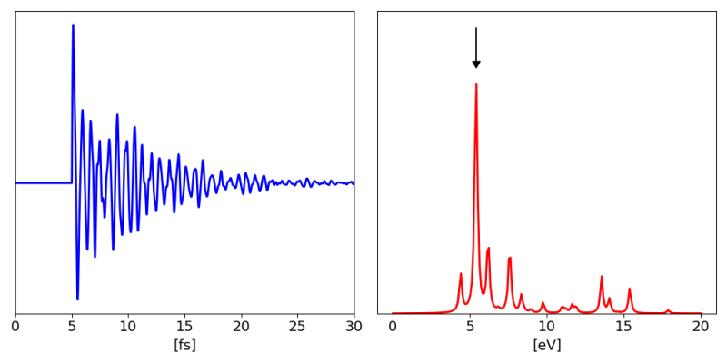
and get the dielectric response. Hereafter we plot the polarization along the y-direction and the corresponding dielectric constant:
Now we start from the previous input cp yambo.in_probe yambo.in_pump and
modify it
in order perform a calculation with the Pump field only: yambo_nl -u p -V nl -F yambo.in_pump. These result will be our reference field in the final analysis:
nloptics                         # [R] Non-linear spectroscopy
% NLBands
 3 |  6 |                           # [NL] Bands range
%
NLverbosity= "high"              # [NL] Verbosity level (low | high)
NLstep= 5.00000           as    # [NL] Time step length
NLtime= 150.000000           fs    # [NL] Simulation Time
NLintegrator= "CRANKNIC"         # [NL] Integrator ("EULEREXP/RK2/RK4/RK2EXP/HEUN/INVINT/CRANKNIC")
NLCorrelation= "SEX"             # [NL] Correlation ("IPA/HARTREE/TDDFT/LRC/LRW/JGM/SEX")
NLLrcAlpha= 0.000000             # [NL] Long Range Correction
NLDamping= 0.000000        eV    # [NL] Damping (or dephasing)
#EvalCurrent                   # [NL] Evaluate the current
HARRLvcs=  913             RL    # [HA] Hartree     RL components
EXXRLvcs=  913             RL    # [XX] Exchange    RL components
% GfnQP_E
 3.594325 | 1.000000 | 1.000000 |        # [EXTQP G] E parameters  (c/v) eV|adim|adim
%
% Field1_Freq
 0.100000 | 0.100000 |         eV    # [RT Field1] Frequency
%
Field1_Int=  1000.00       kWLm2 # [RT Field1] Intensity
Field1_Width= 0.000000     fs    # [RT Field1] Width
Field1_kind= "DELTA"             # [RT Field1] Kind(SIN|RES|ANTIRES|GAUSS|DELTA|QSSIN)
Field1_pol= "linear"             # [RT Field1] Pol(linear|circular)
% Field1_Dir
 0.000000 | 1.000000 | 0.000000 |        # [RT Field1] Versor
%
% Field1_Dir_circ
 0.000000 | 0.000000 | 0.000000 |        # [RT Field1] Versor_circ
%
Field1_Tstart= 165.00000    fs    # [RT Field1] Initial Time
% Field2_Freq
 6.1 | 6.1 |         eV    # [RT Field2] Frequency
%
Field2_Int= 1.E4      kWLm2 # [RT Field2] Intensity
Field2_Width= 10.000000     fs    # [RT Field2] Width
Field2_kind= "QSSIN"              # [RT Field2] Kind(SIN|RES|ANTIRES|GAUSS|DELTA|QSSIN)
Field2_pol= "linear"             # [RT Field2] Pol(linear|circular)
% Field2_Dir
 0.000000 | 1.000000 | 0.000000 |        # [RT Field2] Versor
%
% Field2_Dir_circ
 0.000000 | 0.000000 | 0.000000 |        # [RT Field2] Versor_circ
%
Field2_Tstart= 0.00000    fs    # [RT Field2] Initial Time
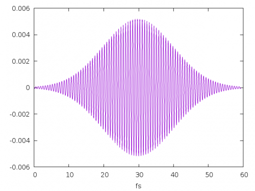
We set the starting time of the Probe (Field1) to 165 fs, a time larger then the simulation run in such a way to have only the Pump(Field2) field. As Pump field we use QSSIN that is an sine-Gaussian wave, with a frequency 6.1 eV centered at the energy of the first exciton, and a width of 10 fs:

