Difference between revisions of "Bulk material: h-BN"
| Line 67: | Line 67: | ||
You are now ready to run Yambo. Check that the databases contain the information you expect: | You are now ready to run Yambo. Check that the databases contain the information you expect: | ||
$ yambo -D | $ yambo -D | ||
[RD./SAVE//ns.db1]------------------------------------------ | [RD./SAVE//ns.db1]------------------------------------------ | ||
Bands : 100 | Bands : 100 | ||
K-points : 14 | K-points : 14 | ||
G-vectors [RL space]: 8029 | G-vectors [RL space]: 8029 | ||
Components [wavefunctions]: 1016 | Components [wavefunctions]: 1016 | ||
... | ... | ||
[RD./SAVE//ns.wf]------------------------------------------- | [RD./SAVE//ns.wf]------------------------------------------- | ||
Fragmentation :yes | Fragmentation :yes | ||
... | ... | ||
[RD./SAVE//ns.kb_pp_pwscf]---------------------------------- | [RD./SAVE//ns.kb_pp_pwscf]---------------------------------- | ||
Fragmentation :yes | Fragmentation :yes | ||
- S/N 006626 -------------------------- v.04.01.02 r.00000 - | - S/N 006626 -------------------------- v.04.01.02 r.00000 - | ||
In practice we suggest to move the <code>SAVE</code> into a new clean folder. | In practice we suggest to move the <code>SAVE</code> into a new clean folder. | ||
Revision as of 13:21, 23 March 2017
In this tutorial you will learn how to generate the Yambo SAVE folder for bulk hBN starting from a PWscf calculation.
Prerequisites
You will need:
- PWSCF input files and pseudopotentials for hBN bulk (Download here)
pw.xexecutable, version 5.0 or laterp2yexecutable
System characteristics
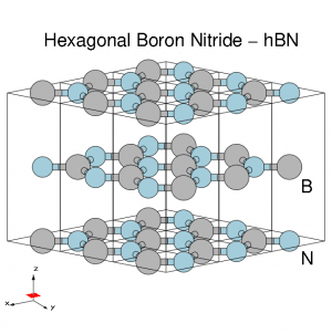
Hexagonal boron nitride - hBN:
- HCP lattice, ABAB stacking
- Four atoms per cell, B and N (16 electrons)
- Lattice constants: a = 4.716 [a.u.], c/a = 2.582
- Plane wave cutoff 40 Ry (1500 RL vectors in wavefunctions)
- SCF run: shifted 6x6x6 grid with 8 bands
- Non-SCF run: unshifted 6x6x2 grid with 100 bands
DFT calculations
Unpack the tarfile. It uses the same file structure as other yambo tutorials:
$ tar -xcvf hBN-bulk.tar
$ cd YAMBO_TUTORIALS/hBN/PWSCF
$ ls
Inputs		Pseudos		PostProcessing		References
hBN_scf.in	hBN_nscf.in     hBN_scf_plot_bands.in  hBN_nscf_plot_bands.in
First run the SCF calculation to generate the ground-state charge density, occupations, Fermi level, and so on:
pw.x < hBN_scf.in > hBN_scf.out
The output reports 36 k-points. The valence band maximum is at 5.13eV.
Next run a non-SCF calculation to generate a set of Kohn-Sham eigenvalues and eigenvectors across a denser k-point mesh, for occupied and unoccupied states:
pw.x < hBN_nscf.in > hBN_nscf.out
Note the presence of the following flags in the input file:
wf_collect=.true.
force_symmorphic=.true.
which are needed for generating the Yambo databases. Full explanations of these variables are given on the quantum-ESPRESSO input variables page.
After these two runs, you should have a hBN.save directory:
$ ls hBN.save
data-file.xml charge-density.dat gvectors.dat B.pz-vbc.UPF N.pz-vbc.UPF
K00001	K00002 .... 	K00035	K00036
Conversion to Yambo format
The PWscf bBN.save output is converted to the Yambo format using the p2y executable (pwscf to yambo), found in the yambo bin directory.
Enter hBN.save and launch p2y:
$ cd hBN.save
$ p2y
...
<---> DBs path set to .
<---> Index file set to data-file.xml
<---> Header/K-points/Energies... done
...
<---> == DB1 (Gvecs and more) ...
<---> ... Database done
<---> == DB2 (wavefunctions)  ... done ==
<---> == DB3 (PseudoPotential) ... done ==
<--->  == P2Y completed ==
This output repeats some information about the system and generates a SAVE directory:
$ ls SAVE
ns.db1  ns.wf  ns.kb_pp_pwscf
ns.wf_fragments_1_1 ...
ns.kb_pp_pwscf_fragment_1 ...
These files, with an n prefix, indicate that they are in netCDF format, and thus not human readable. However, they are perfectly transferable across different architectures.
You are now ready to run Yambo. Check that the databases contain the information you expect:
$ yambo -D
[RD./SAVE//ns.db1]------------------------------------------
Bands                           : 100
K-points                        : 14
G-vectors             [RL space]:  8029
Components       [wavefunctions]: 1016
...
[RD./SAVE//ns.wf]-------------------------------------------
Fragmentation                    :yes
...
[RD./SAVE//ns.kb_pp_pwscf]----------------------------------
Fragmentation                    :yes
- S/N 006626 -------------------------- v.04.01.02 r.00000 -
In practice we suggest to move the SAVE into a new clean folder.
In this tutorial however, we ask instead that you continue using a SAVE we prepared previously:
$ cd ../../YAMBO
$ ls
SAVE
Advanced users
p2y accepts several command line options:
$ p2y -H
dfadsfas
