Difference between revisions of "Bethe-Salpeter"
| Line 20: | Line 20: | ||
To do the Tutorial you have two options: | To do the Tutorial you have two options: | ||
''Option A): Start from the beginning (DFT runs also) | ''Option A): Start from the beginning (DFT runs also) | ||
''Option B): Read directly a prepared SAVE database'' | ''Option B): Read directly a prepared SAVE database'' | ||
| Line 29: | Line 29: | ||
==Option A: Start from the beginning (DFT runs also) == | |||
In this case you will need: | In this case you will need: | ||
| Line 64: | Line 64: | ||
SAVE | SAVE | ||
== Initialization == | ===Initialization=== | ||
As you should know any Yambo run must start with the Initialization step. Simply launch the code | As you should know any Yambo run must start with the Initialization step. Simply launch the code | ||
| Line 76: | Line 75: | ||
==Option B): Read directly a prepared SAVE database== | |||
Note that in this case in the SAVE directory you have already the following databases | Note that in this case in the SAVE directory you have already the following databases | ||
ndb.gops ndb.kindx ndb.RIM ndb.cutoff ndb.pp ndb.QP databases | ndb.gops ndb.kindx ndb.RIM ndb.cutoff ndb.pp ndb.QP databases | ||
Revision as of 14:37, 15 March 2017
UNDER CONSTRUCTION (MP)
In this tutorial you will learn how to:
- generate input files to run a BSE calculation for a two-dimensional material
- run the code and control inputs and outputs
- understand the content of the outputs
Prerequisites
Material: two-dimensional hexagonal BN:
- exagonal lattice
- 2 atoms per cell, B and N (8 electrons)
- Lattice constants: a = 4.716 [a.u.]
- Plane wave cutoff 40 Ry
To do the Tutorial you have two options:
  Option A): Start from the beginning (DFT runs also)
  Option B): Read directly a prepared SAVE database
If you choose Option B) look below for Option B): Read directly a prepared SAVE database and start from there. Please note that in this case you do not need to run the initialization, cutoff generation, calculation of screening W and quasi-particle energies. All the databases ndb.gops ndb,kindx ndb.RIM ndb.cutoff ndb.pp ndb.QP have been already generated for you and are in the SAVE directory
Option A: Start from the beginning (DFT runs also)
In this case you will need:
- PWSCF input files and pseudopotentials for hBN-2D
pw.xexecutable, version 5.0 or laterp2yandyamboexecutables
Unpack the TARFILE:
$ tar -xcvf hBN-2D.tar
Go in the PWSCF directory and list the files.
$ cd hBN-2D/PWSCF
$ ls
hbn-2D_scf.in hbn-2D_nscf.in References tmp
Have a look at the main variables in the inputs hbn-2D_scf.in hbn-2D_nscf.in: k-points, nbnd etc.
Run the DFT self-consistent (scf) and non-self-consistent (nscf) inputs.
$ pw.x < ./Inputs/hbn_2d_scf.in > hbn_2d_scf.out
$ pw.x < ./Inputs/hbn_2d_scf.in > hbn_2d_nscf.out
Generate the SAVE database
$ cd ./tmp/hbn_2d.save
$ p2y
Move the SAVE database in the YAMBO directory to start the calculations with yambo
$ mv  SAVE ../../../YAMBO
$ cd ../../../YAMBO
$ ls
SAVE
Initialization
As you should know any Yambo run must start with the Initialization step. Simply launch the code
$ yambo
This will run the initialization (setup) runlevel.
TIP: do not run yambo from inside the SAVE folder! It will complain that "databases not found".
Option B): Read directly a prepared SAVE database
Note that in this case in the SAVE directory you have already the following databases ndb.gops ndb.kindx ndb.RIM ndb.cutoff ndb.pp ndb.QP databases
$ tar -xcvf hBN-2D.tar $ cd hBN-2D/YAMBO $ mv ./References/SAVE SAVE
Initialization
Every Yambo run must start with this step. Go to the folder containing the hBN-2D SAVE directory:
$ cd TUTORIALS/hBN-2D/YAMBO
$ ls
SAVE
and simply launch the code
yambo
This will run the initialization (setup) runlevel.
TIP: do not run yambo from inside the SAVE folder! It will complain that "databases not found".
BSE Tutorials at present:
- SiH_4
- Fantastic dimension
- LiF
- you Hydrogen
- GaSb (SOC)
- hexagonal BN (on slides only)
The material
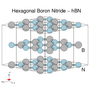
The h-BN is a layered material similar to graphite. It is an indirect wide band-gap material. Its optical spectrum is characterized by large excitonic effects. 5.95 eV is the minimum electronic indirect gap. 6.47 eV is the minimum direct gap. See the literature [1]
|
Bulk hexagonal BN
|
[[File:|Band Structure]] |
Calculate the screening
A key ingredient to construct the BS kernel in the Screeened EXchange approximation (sex) is the screened electron-electron dielectric matrix W which is normally evaluated in the static approximation.
You have two main options to generate the input :
1) yambo -b -F yambo_Ws.in
This will create the input to calculate W (database ndb.em1s)
2) yambo -p p -F yambo_Wp.in
This will create the input to calculate (or read) W in the PPA approximation (database ndb.pp) This second option is useful if you want to read the static part of W from a previous database ndb.pp generated in a GW-PPA run
Calculate the BS kernel in the SEX (Screened Exchange approximation) in the transitions space
Here we learn how to create the BS kernel in the screened exchange (SEX) approximation which includes both exchange (V) and correlation (-W) terms Runlevel to be used yambo -o b -k sex
Solve the BSE by haydock solver and and calculate spectrum
Generate the input file for solving the BSE using the Haydock solver:
yambo -o-y h
Solve the BSE by diagonalizing the excitonic matrix and calculate spectrum
Runlevel to be used yambo -y d
Steps:
-Calculate screening
-Calculate the BS Kernel
-Diagonalize the BS Matrix and calculate spectrum
-Visualize/Analyze excitons (with ypp)
-How to Converge
-How to work with SOC

