Yambopy tutorial: Yambo databases

In this tutorial we will see some examples on how to read and analyse the data contained in the Yambo netCDF databases, which are not readily available as human readable outputs.

In particular we will take a look at:

• Lattice geometry data (Yambo database: ns.db1, Yambopy class: YamboLatticeDB).
• Electron-phonon matrix elements (Yambo databases: ndb.elph_gkkp*, Yambopy class: YamboElectronPhononDB).
• Dipole matrix elements (Yambo databases: ndb.dipoles, Yambopy class: YamboDipolesDB).
• Exciton wavefunctions, energy and spectra (Yambo databases: ndb.BS_diago_Q*, Yambopy class: YamboExcitonDB).

We will also check the command line instructions to quickly generate yambo SAVE folders.

The scripts of the tutorial, but not the databases, can be found in the yambopy directory:

$cd tutorial/databases_yambopy

The full tutorial, including the Quantum espresso and Yambo databases that we will read, can be downloaded and extracted from the yambo website:

$wget https://media.yambo-code.eu/educational/tutorials/files/databases_yambopy.tar.gz
$tar -xvzf databases_yambopy.tar.gz
$cd databases_yambopy

We will work with monolayer hexagonal boron nitride electron-phonon and exciton data obtained on a 12x12x1 kpoint grid. Beware that these are certainly not converged.

Command line: generating the Yambo SAVE

Yambopy offers a set of command line options. In order to review them, you can type

$yambopy

which will print the output

yambopy
Available commands are:

      plotem1s ->     Plot em1s calculation
     analysebse ->     Using ypp, you can study the convergence of BSE calculations in 2 ways:
     analysegw ->     Study the convergence of GW calculations by looking at the change in band-gap value.
  plotexcitons ->     Plot excitons calculation
         addqp ->     Add corrections from QP databases.
       mergeqp ->     Merge QP databases
          save ->     Produce a SAVE folder
          gkkp ->     Produce a SAVE folder including elph_gkkp databases
         bands ->     Script to produce band structure data and visualization from QE.
        serial ->     Script to update serial numbers of yambo ndb.* databases in order to import them to new calculations.
          test ->     Run yambopy tests

For this tutorial, we will need the save and gkkp options. By typing in one of these, additional information about how to run the commands will be printed, e.g.:

$yambopy save

Produce a SAVE folder

Arguments are:
  -nscf, --nscf_dir  -> Path to nscf save folder
  -y, --yambo_dir    -> <Optional> Path to yambo executables

The quantum espresso save for hBN is provided in the directory BSE_saves/QE_saves/hBN.save (you can check the contents of the various folders). Then, following the instructions printed on screen, we can generate a yambo SAVE from the hBN.save by typing

$yambopy save -nscf BSE_saves/QE_saves/hBN.save

This should produce a SAVE folder in the current directory.

Lattice intro: plot k-point coordinates in IBZ/BZ

For this section we will use the script bz_plot.py.

By inspecting the SAVE folder we have just generated, we will find the ns.db1 database which contains all the geometry and lattice information. We are now going to read it in python by using the Yambopy class YamboLatticeDB, which can be instanced like this:

from yambopy import *
ylat = YamboLatticeDB.from_db_file(filename="PATH/TO/SAVE/ns.db1")

(remember to edit the variable save_path in order to point at your yambo SAVE).

The ylat object now contains many useful information as attributes, such as the k-points in Cartesian or crystal coordinates, the system symmetries, lattice constants and basis vectors in real and reciprocal space, etc. The k-points are also automatically expanded in the full Brillouin zone from the irreducible one (you can turn this off with the option Expand=False).

Directly printing the object with

print(ylat)

will also give us some general parameters related to the database.

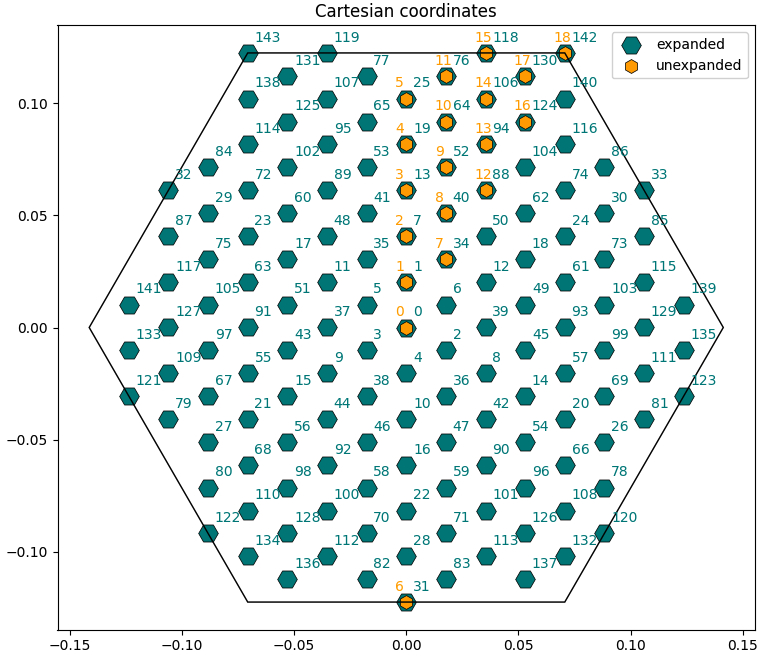
Now check the bz_plot.py script. You will see that it performs three plots:

• Scatterplot of the k-points in Cartesian coordinates with both expanded and unexpanded grids, with annotated indices [Cartesian_Plot=True].
• Scatterplot of the k-points in crystal coordinates [Crystal_Plot=True].
• Manual transformation of a chosen k-point from irreducible to full Brillouin zone (you can change the index i_k in the script to check different cases) [Symmetry_Plot=True].

Dipoles intro: plots of dipoles on BZ, plot of IP absorption

In this section we will use the script dipoles_plot.py and read the dipole databases generated in an optical absorption calculation by yambo. Keep in mind that from now on we will use the "BSE" yambo SAVE generated in the first section.

The databases written after a calculation of optical properties with yambo (dipoles, static screening, excitons) are in the directory BSE_saves/BSE_databases. Here we will also find ndb.dipoles which is needed now, since it contains the matrix elements d_{vck}(\alpha) where vk and ck are the valence and electron states involved in the transition and \alpha the polarisation direction of the external electric field.

In order to read it in python we use the Yambopy class YamboDipolesDB, which can be instanced like this:

ydip = YamboDipolesDB(ylat,save='path/to/BSE/databases',filename='ndb.dipoles')

(notice that it requires a previous instance of YamboLatticeDB).

In addition, in order to read the Kohn-Sham energies, we can also instance the YamboElectronsDB as

yel = YamboElectronsDB(ylat,save='path/to/SAVE')

The object ydip now has a method that permits to retrieve the independent-particle absorption spectrum with customly chosen energy range, steps, and broadening:

w, eps2 = ydip.ip_eps2(yel)

In order to see all this in action, take a look at the dipoles_plot.py script. You will see that it performs two plots:

• Plot of |d(k)| in the BZ for selected v,c and \alpha (we choose the layer plane 'xy') [Kspace_Plot=True]. From this plot you can appreciate which sections of the BZ contribute the most to the absorption rate.
• Plot of the independent-particles absorption spectrum [Absorption_Plot=True].

You can play with the indices and the plot parameters to check what happens.

Exciton intro 1: read and sort data

In this section we will use the script exc_read.py and read the exciton data resulting from a BSE calculation in order to familiarise with their structure. This time we are going to read the ndb.BS_diago_Q* databases which correspond to BSE calculations at various momenta Q (Q=1 being the zero-momentum optical absorption limit - notice that python indexing starts from 0, while the databases are counted starting from 1).

In order to read them in python we use the Yambopy class YamboExcitonDB, which can be instanced like this:

yexc = YamboExcitonDB.from_db_file(ylat,filename='path/to/BSE/databases/ndb.BS_diago_Q%d'(i_Q+1))

(notice that it requires a previous instance of YamboLatticeDB).

Now the yexc object contains information about the exciton energies (yexc.eigenvalues), wave functions (yexc.eigenvectors) and intensities (yexc.l_residuals, yexc.r_residuals) for Qpoint i_Q. You can start by keeping Q1 which is the optical limit and then check other momenta.

The exciton wave function components A_{vck}^{\lambda Q} (\lambda being the exciton index) are stored as A_{t}^{\lambda} in each Q-dependent database, with t being the transition index grouping the single-particle indices vck. Therefore, yexc.eigenvectors is an array with (N_excitons,N_transitions) dimension. In order to make the connection t->kcv, the table yexc.table provides k,v,c and spin indices corresponding to each transition.

In order to get a clearer picture, take a look at the script exc_read.py. Run it and try to understand the outputs.

 $ python exc_read.py

Exciton intro 2: plot exciton weights on k-BZ and (interpolated) band structure

In this section we will use the script exc_kspace_plot.py and work with the quantities defined in the previous section.

For now, only the i_Q=0 case is implemented in this section. We want to check the relative importance of the various (vk->ck) electronic transitions in forming a certain excitonic state.

Since many excitonic states are degenerate, we first need to tell Yambopy which states we want to check. For example, in monolayer hexagonal boron nitride, the lowest-bound exciton - forming the main peak in the BSE absorption spectrum - is doubly degenerate. In order to analyse it, in the exc_kspace_plot.py script we set

states = [1,2]

(we can also set [3,4] to check the second excitonic state, and then [5] for the non-degenerate third state, and so on; we can check degeneracies by printing the energies using the script exc_read.py).

In order to make a band structure plot, it is necessary to read the band energies, for example with the YamboSaveDB class

yel = YamboSaveDB.from_db_file(folder='path/to/SAVE')

and specify the path in the BZ using crystal coordinates via the Path function:

npoints = 20
path = Path([ [[  0.0,  0.0,  0.0],'$\Gamma$'],
              [[  0.5,  0.0,  0.0],'M'],
              [[1./3.,1./3.,  0.0],'K'],
              [[  0.0,  0.0,  0.0],'$\Gamma$']],
              [int(npoints*2),int(npoints),int(sqrt(5)*npoints)] )

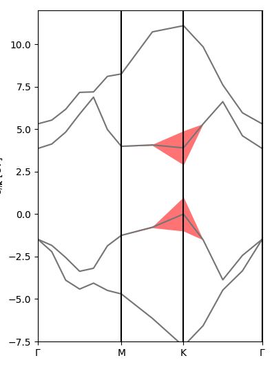
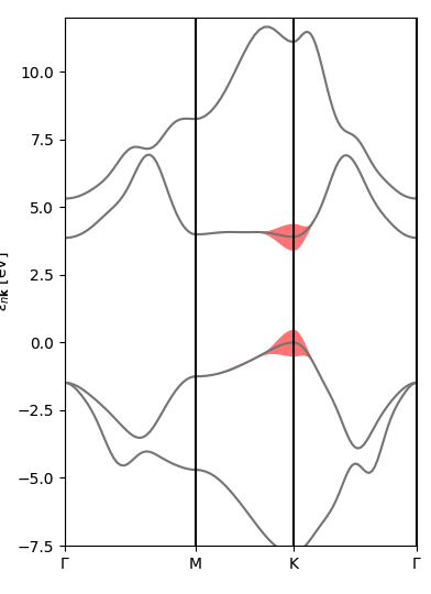
Now let's take a closer look at the exc_kspace_plot.py script. You will see that it performs three plots:

• Plot of |A(k)| in the k-BZ for the selected exciton state. You can see how most contributions come from the area around K and the MK direction [Kspace_Plot=True].
• Plot of |A(v,c,k)| on the electronic band structure for the selected exciton state. Here you can better see how the top valence and bottom conduction around MK are mostly involved [Bands_Plot=True].
• Plot of interpolated |A(v,c,k)| on the interpolated electronic band structure for the selected exciton state [Bands_Plot_Interpolated=True].

As always, try to play with the parameters, for example by changing the excitonic states to analyse.

Exciton intro 3: plot BSE optical absorption with custom options

In this section we will use the script exc_abs_plot.py and work with the quantities defined in the previous sections.

The class YamboExcitonDB also enables us, of course, to read the dielectric function eps(w) and print absorption and related spectra in python.

The advantages over using the standard human-readable yambo outputs are mainly two:

1. We can freely select energy ranges, energy steps, peak broadenings and number of excitonic states included without having to rerun the yambo executable every time. This reduces the chance of mistakenly editing the yambo input and allows for greater freedom since these plots can now be done in your local machine without having to transfer the output data from a remote cluster.
2. The dielectric function constructed from netCDF database variables has a much higher precision (number of significant digits) than the human readable output, which may be important if you want to perform additional operations in python (e.g., computing refractive index, reflectivity and other optical spectra from it, performing finite-difference derivatives, etc).

We can read eps(w) as a numpy array with the specified options as (energy values are in eV):

w, eps = yexc.get_chi(nexcitons='all',emin=0,emax=7,estep=0.005,broad=0.04)

Or, you can directly prepare a plot of its imaginary part with

w, chi = yexc.plot_chi_ax(ax,nexcitons='all',emin=0,emax=7,estep=0.005,broad=0.04)

where ax is a previously defined Axes object from matplotlib.

In order to see how this works, let's take a look at the exc_abs_plot.py script. You will see that it performs the two operations described above:

• Plotting the BSE absorption spectrum [Absorption_Plot=True].
• Reading the complex dielectric function.

Try to customise the plots by changing the nexcitons, emin, emax, estep, broad parameters.

Command line: importing electron-phonon matrix elements

You may have seen how to calculate and import electron-phonon matrix elements in yambo in the electron-phonon tutorial.

With Yambopy, we can generate a yambo SAVE folder and import the matrix elements with a single command. Typing

$yambopy gkkp

will print the necessary documentation:

Produce a SAVE folder including elph_gkkp databases

Arguments are:
  -nscf, --nscf_dir  -> <Optional> Path to nscf save folder
  -elph, --elph_dir  -> Path to elph_dir folder
  -y, --yambo_dir    -> <Optional> Path to yambo executables
  -e, --expand       -> <Optional> Expand gkkp databases

The necessary quantum espresso databases are stored in ELPH_SAVES/QE_SAVES/hBN.save (nscf calculation) and ELPH_SAVES/QE_SAVES/elph_dir (matrix elements from the dfpt calculation). For this tutorial we also need to expand the electron-phonon matrix elements to the full Brillouin zone. Since this is a different calculation with respect to the previous section, please generate this SAVE in a different directory than the one you used for the previous SAVE, which should be the current directory. For example:

$mkdir yambo-with-elph
$cd yambo-with-elph

Now we can run yambopy as in the instructions:

$yambopy gkkp -nscf ../ELPH_saves/QE_saves/hBN.save -elph ../ELPH_saves/QE_saves/elph_dir --expand

This should generate a yambo SAVE folder which contains the ndb.elph_gkkp_expanded* databases.

Electron-phonon intro: plots of el-ph matrix elements on k-BZ and q-BZ

In this section we will use the script elph_plot.py and read the electron-phonon databases that you generated in the previous section.

In order to read the ndb.elph_gkkp_expanded* databases in python we use the Yambopy class YamboElectronPhononDB, which can be instanced like this:

yelph = YamboElectronPhononDB(ylat,folder_gkkp='path/to/elph/folder',save='path/to/SAVE')

(notice that it requires a previous instance of YamboLatticeDB).

Now, the yelph object contains phonon frequencies, phonon eigenvectors, qpoint information and, of course, the electron-phonon matrix elements g_{nm\nu}(k,q) where n, m are electron band states, \nu is a phonon branch, and k and q are the electronic and transfer momenta.

We can print the docstring of the YamboElectronPhononDB class with

print(yelph.__doc__)

to get an idea of the information stored and of its capabilities.

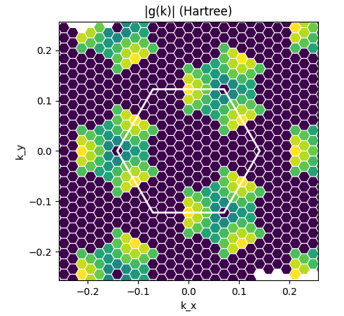
Now check the elph_plot.py script. You will see that it performs two plots:

• Plot of |g(k)| in the k-BZ for selected n,m,\nu and q [Kspace_Plot=True].
• Plot of |g(q)| in the q-BZ for selected n,m,\nu and k [Qspace_Plot=True].

You can change the electronic, phononic and momentum indices to see what happens.

Links

• Back to Rome 2023#Tutorials
• Back to ICTP 2022#Tutorials