Angular dependence of non-linear response

Introduction
In this tutorial we show how to calculate angular dependence of non-linear response using Yambo. (This tutorial requires Yambo >= 5.3)
We consider as example a monolayer hBN, DFT input files can be downloaded here: hBN-2D-RT.tar.gz
In this tutorial we suppose you already know how to calculate non-linear reponse with Yambo,
if this is not the case please have a look to the tutorials: Non linear response
Run DFT calculation, import the wave-function and run the setup. Then we can start:
Remove symmetries
We remove all symmetries Using the command ypp_nl -y
fixsyms
# [R] Remove symmetries not consistent with an external perturbation
% Efield1
  0.000000 | 0.000000 | 0.000000 |   # First external Electric Field
%
% Efield2
 0.000000 | 0.000000 | 0.000000 |      # Additional external Electric Field
%
BField= 0.000000           T     # [MAG] Magnetic field modulus
Bpsi= 0.000000             deg   # [MAG] Magnetic field psi angle [degree]
Btheta= 0.000000           deg   # [MAG] Magnetic field theta angle [degree]
RmAllSymm                  # Remove Time Reversal
notice that in principle one could remove only the symmetries of the rotation plane plus the TimeReversal.
Then go in the FixSymm folder and run the setup again
Run a standard SHG calculation
We first run a SHG calculation using the input
nloptics                         # [R] Non-linear spectroscopy
% NLBands
   3 | 6 |                           # [NL] Bands range
%
NLverbosity= "high"              # [NL] Verbosity level (low | high)
NLtime=-1.000000           fs    # [NL] Simulation Time
NLintegrator= "INVINT"           # [NL] Integrator ("EULEREXP/RK2/RK4/RK2EXP/HEUN/INVINT/CRANKNIC")
NLCorrelation= "IPA"             # [NL] Correlation ("IPA/HARTREE/TDDFT/LRC/LRW/JGM/SEX")
NLLrcAlpha= 0.000000             # [NL] Long Range Correction
% NLEnRange
   1.000000 |6.000000 |         eV    # [NL] Energy range
%
NLEnSteps=  160                    # [NL] Energy steps
NLDamping= 0.200000        eV    # [NL] Damping (or dephasing)
RADLifeTime=-1.000000      fs    # [RT] Radiative life-time (if negative Yambo sets it equal to Phase_LifeTime in NL)
% Field1_Freq
 0.100000 | 0.100000 |         eV    # [RT Field1] Frequency
%
Field1_NFreqs= 1                 # [RT Field1] Frequency
Field1_Int=  1000.00       kWLm2 # [RT Field1] Intensity
Field1_Width= 0.000000     fs    # [RT Field1] Width
Field1_kind= "SOFTSIN"           # [RT Field1] Kind(SIN|COS|RES|ANTIRES|GAUSS|DELTA|QSSIN)
Field1_pol= "linear"             # [RT Field1] Pol(linear|circular)
% Field1_Dir
  0.000000 | 1.000000 | 0.000000 |        # [RT Field1] Versor
%
Field1_Tstart= 0.010000    fs    # [RT Field1] Initial Time
from this run we get the X2yyy(ω) spectrum:

where we put an arrow at 2.45 eV, the frequency where we want to study the angula dependence of the SHG. Notice that this specrum is not a converged one due to the small k-point grid and the reduced number of bands.
Run SHG at different angles
Using the same command yambo_nl -u n to generate the input at different angles:
nloptics                         # [R] Non-linear spectroscopy
% NLBands
   3 |  6 |                           # [NL] Bands range
%
NLverbosity= "high"              # [NL] Verbosity level (low | high)
NLtime=-1.000000           fs    # [NL] Simulation Time
NLintegrator= "INVINT"           # [NL] Integrator ("EULEREXP/RK2/RK4/RK2EXP/HEUN/INVINT/CRANKNIC")
NLCorrelation= "IPA"             # [NL] Correlation ("IPA/HARTREE/TDDFT/LRC/LRW/JGM/SEX")
NLLrcAlpha= 0.000000             # [NL] Long Range Correction
% NLEnRange
-1.000000 |-1.000000 |         eV    # [NL] Energy range (for loop on frequencies NLEnSteps/=0
%
NLEnSteps=0                      # [NL] Energy steps for the loop on frequencies
% NLrotaxis
  0.000000 | 0.000000 | 1.000000 |        # [NL] Rotation axis (for the loop on angles NLAngSteps/=0)
%
NLAngSteps= 80                     # [NL] Angular steps (if NLAngSteps/=0 field versor will be ignored)
NLDamping= 0.200000        eV    # [NL] Damping (or dephasing)
RADLifeTime=-1.000000      fs    # [RT] Radiative life-time (if negative Yambo sets it equal to Phase_LifeTime in NL)
% Field1_Freq
  2.450000 | 2.450000 |         eV    # [RT Field1] Frequency
%
Field1_NFreqs= 1                 # [RT Field1] Frequency
Field1_Int=  1000.00       kWLm2 # [RT Field1] Intensity
Field1_Width= 0.000000     fs    # [RT Field1] Width
Field1_kind= "SOFTSIN"           # [RT Field1] Kind(SIN|SOFTSIN| see more on src/modules/mod_fields.F)
Field1_pol= "linear"             # [RT Field1] Pol(linear|circular)
% Field1_Dir
  0.000000 | 1.000000 | 0.000000 |        # [RT Field1] Versor
%
Field1_Tstart= 0.010000    fs    # [RT Field1] Initial Time
In this input we ask to Yambo to rotate the laser vector around the z-axis, NLrotaxis = 0.000000 | 0.000000 | 1.000000 .
Starting from the vector in the plane Field1_Dir=0.000000 | 1.000000 | 0.000000.
Thefore 0-degree means y-direction, while 90-degree is equivalent to x-direction.
The laser frequency is specified in the field Field1_Freq, in our case 2.5 eV.
When you run the code, Yambo will generate 80 angles (NLAngSteps) between 0 and 360 degrees and perform the calculations for each angle.
The result can be analysed with the same SHG tools, namely the command ypp_nl -u n:
nonlinear                        # [R] Non-linear response analysis
Xorder=    4                        # Max order of the response/exc functions
% TimeRange
 39.49271 | -1.00000 |         fs    # Time-window where processing is done
%
ETStpsRt= 200                    # Total Energy steps
% EnRngeRt
  0.00000 | 20.00000 |         eV    # Energy range
%
DampMode= "NONE"                 # Damping type ( NONE | LORENTZIAN | GAUSSIAN )
DampFactor= 0.000000       eV    # Damping parameter
PumpPATH= "none"                 # Path of the simulation with the Pump only
the code will produce a series of files o.YPP-X_angle_order_x where "x" is the order of the response function. The file contains the results at the different angles in the form:
#    Angle [grad]       X/Im[cm/stV](x)    X/Re[cm/stV](x)    X/Im[cm/stV](y)    X/Re[cm/stV](y)    X/Im[cm/stV](z)    X/Re[cm/stV](z)
#
     0.0000000        -0.28935743E-08    -0.49004950E-09     0.26119386E-06    -0.16474487E-07      0.0000000          0.0000000
     4.50000000        0.410850702E-7    -0.154496459E-8     0.255967326E-6    -0.169618359E-7      0.00000000         0.0000000
     9.00000000        0.842866430E-7    -0.246935349E-8     0.244313674E-6    -0.171142064E-7      0.00000000         0.0000000
     13.5000000        0.125646460E-6    -0.323807280E-8     0.226519776E-6    -0.169275451E-7      0.00000000         0.0000000
...
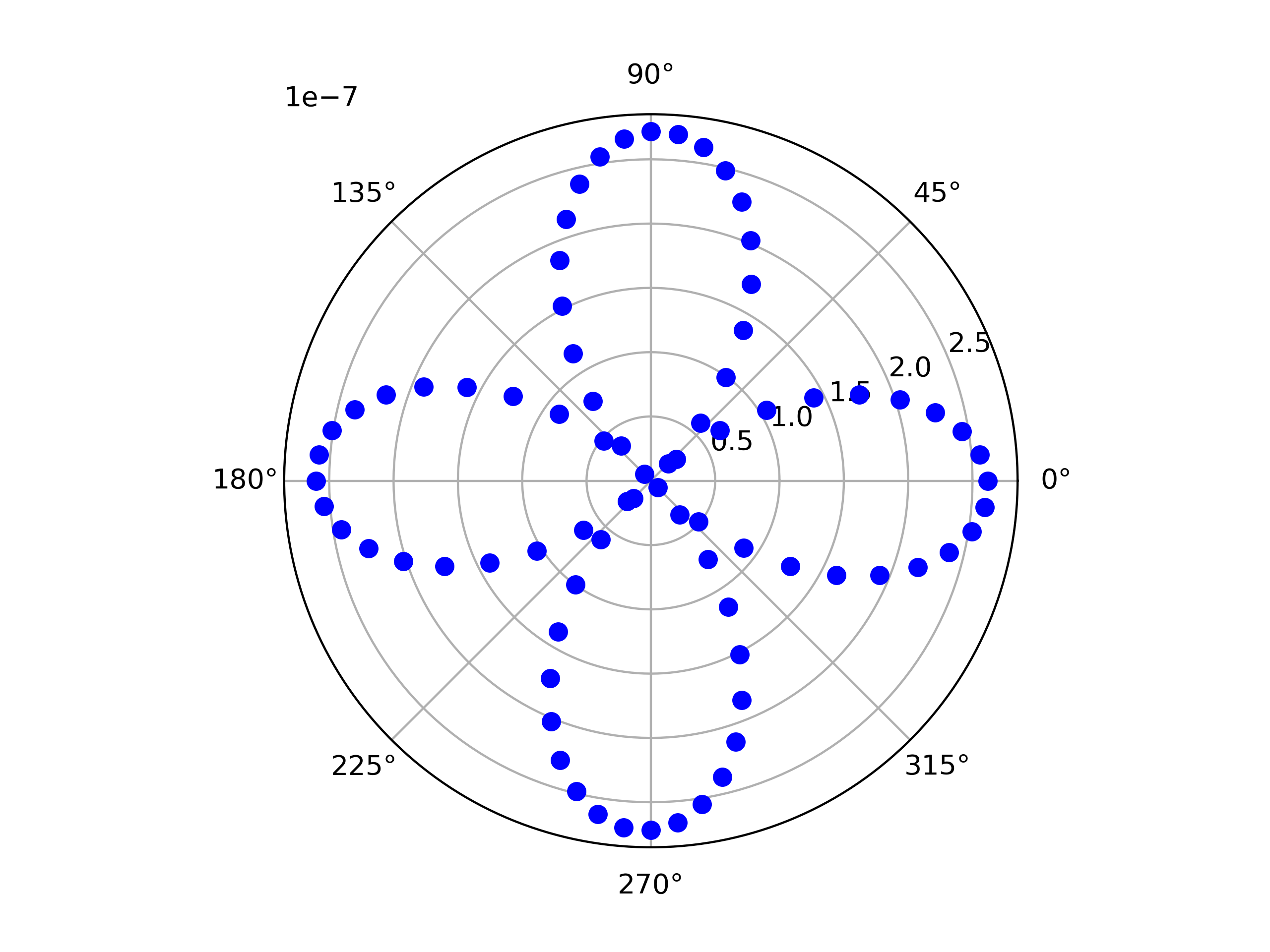
Results can be easily plot with a simple python script as the following one:
import numpy as np
from scipy import signal
import matplotlib.pyplot as plt
from matplotlib.colors import LogNorm
import math as m
fig, ax = plt.subplots(ncols=1,nrows=1,subplot_kw={'projection': 'polar'})
plt.subplots_adjust(hspace=0.6)
data=np.genfromtxt("o.YPP-X_angle_order_2",comments="#")
for iangle in range(0,len(data[:,0])):
    ax.plot(data[iangle,0]/360*(2.0*m.pi),np.sqrt(data[iangle,3]**2+data[iangle,4]**2),'bo:')
plt.savefig('SHG_angle.png',dpi=400)
plt.show()
and hereafter the final result:

Analyze data with YamboPy
Similar to the other tutorials, data analysis can be performed also using YamboPy instead of ypp_nl.

Using the same script to read the database:
from yambopy import *
NLDB=YamboNLDB(calc='ANGLES')
pol =NLDB.Polarization[0]
time=NLDB.IO_TIME_points
Harmonic_Analysis(NLDB,X_order=4)
and then you can plot them:
import numpy as np
from scipy import signal
import matplotlib.pyplot as plt
from matplotlib.colors import LogNorm
import math as m
fig, ax = plt.subplots(ncols=1,nrows=1,subplot_kw={'projection': 'polar'})
plt.subplots_adjust(hspace=0.6)
data=np.genfromtxt("o.YamboPy-X_probe_order_2",comments="#")
for iangle in range(0,len(data[:,0])):
    ax.plot(data[iangle,0]/360*(2.0*m.pi),np.sqrt(data[iangle,3]**2+data[iangle,4]**2),'bo:')
plt.savefig('SHG_angle.png',dpi=400)
plt.show()