Pushing convergence in parallel
This modules contains very general discussions of the parallel environment of Yambo. Still the actual run of the code is specific to the CECAM cluster. If you want to run it just replace the parallel queue instructions with simple MPI commands.
Files and Tools
Database and tools can be downloaded here:
- hBN-2D-para.tar.gz
- parse_ytiming.py (or wiki version: parse_ytiming.py)
- parse_qp.py (or wiki version: parse_qp.py)
2D hBN
In the previous session we focused on the scaling properties of the code. We now focus more on the physical aspect.
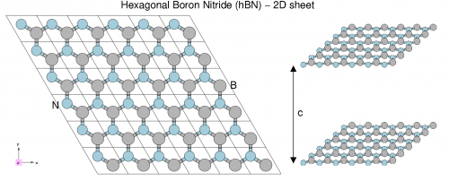
The system we are working on is the 2D-hBN sheet we already used the first day.
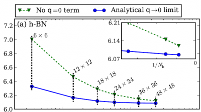
If you want a published reference of quasi-particle properties of hBN you can have a look to the following arxiv, https://arxiv.org/abs/1511.00129 (Phys. Rev. B 94, 155406 (2016)), and references therein, were the GW correction are computed. In that case the convergence with the number of k-points is studied in detail (for hBN and other materials). The focus is on a proper description of the q->0 limit of the (screened) electron-electron interaction entering the GW self-energy. As you can see from the below image extracted from the arxiv the QP corrections converge slowly with the number of k-points.
In the present tutorial you will start using a 12x12 grid. Only in the last part we will re-run pw.x (optional) to generate bigger k-grids
Tomorrow you will learn how to do that in a more automatic way using the yambopy scripting tools, however running yambo in serial. While yambopy offers an easier interface for the use, in the present parallel tutorial you will be able to push much more the convergence. In a real life calculation you will likely take advantage of both.
As this morning if you are not inside bellatrix, please follow the instructions in the tutorial home. If you are inside bellatrix and in the proper folder
[cecam.school01@bellatrix yambo_YOUR_NAME]$ pwd
/scratch/cecam.schoolXY/yambo_YOUR_NAME
you can proceed.
$ cd YAMBO_TUTORIALS/hBN-2D-para/YAMBO
For the present tutorial you will need an upgraded version of the parse_qp.py.
You can get it from the scratch folder
$ cp /scratch/cecam.school/parse_qp.py ./
Convergence on the number of bands in X and G
To do convergence calculations you need to execute the same run many time, progressively changing one (or more of the input variables) We start considering the number of bands entering the construction of the response function. This will then be used to compute the screened electron-electron interaction, W, needed for the GW self-energy.
% BndsRnXp
    1 |  200 |               # [Xp] Polarization function bands
%
Try to use different values, going to a very small one (say 10) up to the maximum allowed by the number of bands computed with pw.x to generate the present database (400). You may use 10, 25, 50, 100, 200, 400. Since now the focus is not anymore on the number of cores but on the yambo input parameters, it is a good idea to label the jobname accordingly to the latter in the run.sh script:
label=Xnb200_Gnb200_ecut4Ry
Then you can use the parse_qp.py script to extract the direct gap using the command
./parse_qp.py run*/o-*.qp
The output should be something similar to
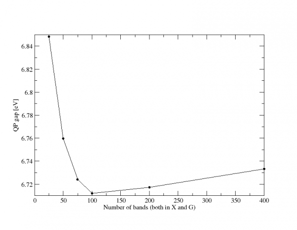
  # Xo_gvect     Xo_nbnd      G_nbnd   Egap [eV]
        245          25          25    6.848440
        245          50          50    6.759580
        245          75          75    6.724210
        245         100         100    6.712120
        245         200         200    6.717220
        245         400         400    6.733410
Now you can try to do the same with the number of bands entering the definition of the green function
% GbndRnge
    1 |  200 |               # [GW] G[W] bands range
%
You can do the same numbers we tried for the bands entering the response function. It is also a good idea to let yambo read the screening from a previous run. To this end you need to create a folder and copy there the screening DB
$ mkdir SCREENING_400bands
$ cp Xnb400_Gnb200_ecut4Ry/ndb.pp* SCREENING_400bands
Then, to let yambo read it, edit the job.sh script creating the new variable
auxjdir=SCREENING_400bands
and
srun -n $ncpu -c $nthreads $bindir/yambo -F $filein -J "$jdir,$auxjdir" -C $cdir
Below how your QP gap should converge versus the total number of band used both in X and G
tips:
- remember to run in parallel, we suggest you keep using 16 cores, with 2 OpenMP threads, but for the biggest runs you can try to use even more than one node
Convergence with the energy cut-off on the response function
The variable we now consider is the energy cut-off, i.e. the number of G-vectors used to construct the [math]\displaystyle{ \chi_{G,G'}(\omega) }[/math] matrix
NGsBlkXp= 4000 mRy # [Xp] Response block size
Even in this case try changing the input value from a low value to a big one. Try 0 (it means the code will just use 1 G vector), 1, 2, 4 and 8. This time you are re-computing the screening, so you cannot use anymore the auxdir from the previous run. just change the script back as
#srun -n $ncpu -c $nthreads $bindir/yambo -F $filein -J "$jdir,$auxjdir" -C $cdir
srun -n $ncpu -c $nthreads $bindir/yambo -F $filein -J $jdir -C $cdir
Convergence with the number of k-points (optional)
For this last step you need to re-run pw.x Go to the DFT folder
$ cd ../PWSCF
$ ls
hBN_2D_nscf.in  hBN_2D_scf.in  Inputs  Pseudos  References
You now need to run pw.x, first the scf step, then then NSCF step.
For the SCF step copy the submit script you used for yambo here,
$ cp ../YAMBO/run.sh ./
change it (you can erase many lines)
$ vim run.sh #!/bin/bash #SBATCH -N 1 #SBATCH -t 06:00:00 #SBATCH -J test_braun #SBATCH --reservation=cecam_course #SBATCH --tasks-per-node=16nodes=1nthreads=8ncpu=`echo $nodes $nthreads 16 | awk '{print $1*$3/$2}'`module purge module load intel/16.0.3 module load intelmpi/5.1.3 bindir=/home/cecam.school/bin/ export OMP_NUM_THREADS=1label=MPI${ncpu}_OMP${nthreads}jdir=run_${label}cdir=run_${label}.outfilein0=yambo_gw.infilein=yambo_gw_${label}.incp -f $filein0 $fileincat >> $filein << EOFX_all_q_CPU= "1 1 $ncpu 1" # [PARALLEL] CPUs for each roleX_all_q_ROLEs= "q k c v" # [PARALLEL] CPUs roles (q,k,c,v)X_all_q_nCPU_LinAlg_INV= $ncpu # [PARALLEL] CPUs for Linear AlgebraX_Threads= 0 # [OPENMP/X] Number of threads for response functionsDIP_Threads= 0 # [OPENMP/X] Number of threads for dipolesSE_CPU= " 1 1 $ncpu" # [PARALLEL] CPUs for each roleSE_ROLEs= "q qp b" # [PARALLEL] CPUs roles (q,qp,b)SE_Threads= 0EOFecho "Running on 16 MPI, 1 OpenMP threads" srun -n 16 -c 1 $bindir/pw.x < hBN_2D_scf.in > hBN_2D_scf.out
and use it
./run.sh
To run the NSCF step first of all open
$ vim hBN_2D_nscf.in
and change the input fil
&control
    calculation='nscf',
    prefix='hBN_2D_kx16',
    pseudo_dir = './Pseudo'
    wf_collect=.true.
    verbosity = 'high'
/
&system
    ibrav = 4,
    celldm(1) = 4.716
    celldm(3) = 7.
    nat= 2,
    ntyp= 2,
    force_symmorphic=.true.
    ecutwfc = 40,nbnd = 400
/
&electrons
   diago_thr_init=5.0e-6,
   diago_full_acc=.true.
   electron_maxstep = 100,
   diagonalization='cg'
   mixing_mode = 'plain'
   mixing_beta = 0.6
   conv_thr =  1.0d-8,
/
ATOMIC_SPECIES
 B 10 B.pz-vbc.UPF
 N 14 N.pz-vbc.UPF
ATOMIC_POSITIONS {crystal}
B  0.6666667  0.3333333  0.0000000
N -0.6666667 -0.3333333  0.0000000
K_POINTS (automatic)
16 16 1 0 0 0
copy the scf density into a new save folder and run pw.x
$ mkdir hBN_2D_kx16.save
$ cp hBN_2D.save/* hBN_2D_kx16.save
(ignore the warning message about the K00* folders) open
$ vim run.sh
modify the submission script
srun -n 16 -c 1 $bindir/pw.x < hBN_2D_nscf.in > hBN_2D_nscf_kx16.out
and run it
$ ./run.sh
You just created the wave-functions on the kx16 grid. Next step is to convert to the Yambo format
$ cd hBN_2D_nscf_kx16.save
$ p2y
$ mkdir ../../YAMBO_kx16
$ mv SAVE ../../YAMBO_kx16
$ cd ../../YAMBO_kx16
$ cp ../YAMBO/run.sh ./
And you are ready to run calculation in the kx16 folder. You may need to repeat the same for smaller and/or bigger k-grids to properly check the convergence against k-points.
| Prev: Tutorials Home | Now: Tutorials Home --> GW Convergence | Next: Parallel tutorials are over |


