LiF
Solid LiF: excitons at work
The material
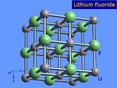
- FCC lattice
- Two atoms per cell, Li and F (8 electrons)
- Lattice constant 7.61 [a.u.]
- Plane waves cutoff 40 Hartree (1800 RL vectors)
The Tutorial files
Follow the instructions in Tutorials#Files and download/unpack the LiF.tar.gz.
From PWscf to the Yambo core databases
$ cd YAMBO_TUTORIALS/LiF/PWSCF
$ ls
inputs	outputs  psps
First run the SCF calculation to generate the ground-state charge density, occupations, Fermi level, and so on:
$ pw.x < inputs/scf.in > scf.out
Next run a non-SCF calculation to generate a set of Kohn-Sham eigenvalues and eigenvectors for both occupied and unoccupied states (100 bands):
$ pw.x < inputs/nscf.in > nscf.out
Note the presence of the following flags in the input file:
wf_collect=.true.
force_symmorphic=.true.
diago_full_acc=.true.
which are needed for generating the Yambo databases accurately. Full explanations of these variables are given on the quantum-ESPRESSO input variables page.
After these two runs, you should have a LiF.save directory:
$ ls LiF.save
charge-density.dat  data-file-schema.xml  F.LDA.cpi.UPF  Li.LDA.cpi.UPF  wfc10.dat  wfc1.dat  wfc2.dat	wfc3.dat  wfc4.dat  wfc5.dat  wfc6.dat	wfc7.dat  wfc8.dat  wfc9.dat
Conversion to Yambo format
The PWscf LiF.save output is converted to the Yambo format using the p2y executable (pwscf to yambo), found in the yambo bin directory.
Enter LiF.save and launch p2y:
$ cd LiF.save
$ p2y
...
<---> DBs path set to .
<---> Index file set to data-file.xml
<---> Header/K-points/Energies... done
...
<---> == DB1 (Gvecs and more) ...
<---> ... Database done
<---> == DB2 (wavefunctions)  ... done ==
<---> == DB3 (PseudoPotential) ... done ==
<--->  == P2Y completed ==
This output repeats some information about the system and generates a SAVE directory:
$ ls SAVE
ns.db1  ns.wf  ns.kb_pp_pwscf
ns.wf_fragments_1_1 ...
ns.kb_pp_pwscf_fragment_1 ...
These files, with an n prefix, indicate that they are in netCDF format, and thus not human readable. However, they are perfectly transferable across different architectures.
In practice we suggest to move the SAVE folder into a new clean folder.
In this tutorial however, we ask instead that you continue using a SAVE folder that we prepared previously:
$ cd ../../Optics/YAMBO
$ ls
SAVE
Introduction
We will start the TDDFT tutorial exactly where standard local approximations for fxc (like ALDA) do not work at all. The optical spectrum of solid LiF [1] is dominated by a strongly bound exciton (3 eV binding energy) [2] and will immediately see that any independent particle approximation drastically fails to describe the complex structures that are observed experimentally.
In the following we will describe in detail the different TDDFT related calculations. For each example you can find a link to the Input file with a brief explanation of the variables meaning.
We will also use this first system to explain in detail some of the most relevant technical aspects of yambo.
Initialization (yambo -i -V RL)
This section describes the standard initialization procedure. As this initialization is common to all yambo runs it will be described extensively only in this case.
To run this example enter the YAMBO directory (where you have previously created the SAVE folder) and type:
localhost:>yambo -F Inputs/01_init -J 01_init
and you will see
 <---> [01] Game Summary
 <---> [02] Input variables setup
 <---> RL-shells |                    | [000%] --(E) --(X)
 <---> RL-shells |####################| [100%] --(E) --(X)
 <---> [02.01] K-grid lattice
 <---> [02.02] Input (E)nergies[ev] & Occupations
 <---> [03] Transferred momenta grid: Indexes
 <---> [04] Game Over & Game summary
If now you edit the r-01_setup you will find a lot of useless (![]() ) informations about your system like, the Fermi level
) informations about your system like, the Fermi level
   [02.02] Input (E)nergies[ev] & Occupations
  ========

  Fermi Energy[ev] - T[ev/K] :-0.241627  0.000100  1.160400
  Bands summary              : Full        Empty
                               0001-0004   0005-0050
  Indirect Gap  [ev][min-max]:  9.11330  14.79631
confirming that, yes, our bulk LiF is a wide gap insulator. Then you can see the effect of using
MaxGvecs= 800 RL # [INI] Max number of G-vectors planned to use
in the Inputs/01_init file. In the report file we notice that
  G-vectors             [RL space]: 1807
                   [wavefunctions]: 1807
whereas the Reciprocal Space shells found by yambo are
 G-vector (S)hells. Format: [Snn] G`s
  [S0030]:   773 [S0029]:   749 [S0028]:   725 [S0027]:   701 [S0026]:   645
  [S0025]:   609 [S0024]:   561 [S0023]:   537 [S0022]:   531 [S0021]:   459
  [S0020]:   411 [S0019]:   387 [S0018]:   339 [S0017]:   331 [S0016]:   307
  [S0015]:   283 [S0014]:   259 [S0013]:   229 [S0012]:   181 [S0011]:   169
  [S0010]:   137 [S0009]:   113 [S0008]:    89 [S0007]:    65 [S0006]:    59
  [S0005]:    51 [S0004]:    27 [S0003]:    15 [S0002]:     9 [S0001]:     1
so that the highest number of RL vectors we can use is 773, lower than the charge number given by Abinit and different from the value for MaxGvecs we provided. This happens because yambo has calculated the Reciprocal Space shells up to 800 to find that the highest closed shell corresponds to 773 RL vectors. Note that, independently of the value you set for any variable that defines a dimension in the RL space, yambo redefines it, in order to match it to the nearest closed shell.
Random-Phase approximation (yambo -o c) (yambo -o c -k hartree) (yambo -o c -k hartree -V qp)
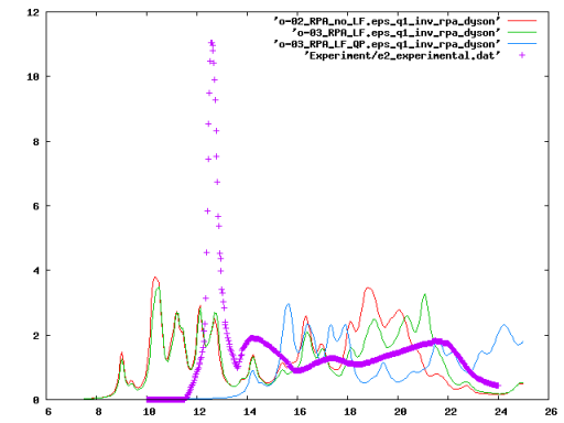
The simplest approximation that can be used to calculate the absorption spectrum of LiF is the independent particle approximation. This is done in Inputs/02_RPA_no_LF, that is generated directly by "yambo -o c" command line without specifying an approximation for the kernel (in fact there is no kernel!), To run this example type
localhost:>yambo -F Inputs/02_RPA_no_LF -J 02_RPA_no_LF
The optional -J flag is used to label the output/report/log files. In Inputs/03_RPA_LF we include a kernel in the Hartree approximation. This correspond to the Random-Phase-Approximation (RPA). The response function size is changed to 51 RL. This means including Local Field Effects corresponding to charge oscillations expanded up to the 51st RL component. The converged value for NGsBlkXd shall be determined by doing several calculations with different values and checking the effect on the final physical result (the absorption spectrum, in this case).
After having run
localhost:>yambo -F Inputs/03_RPA_LF -J 03_RPA_LF
we can compare the result of our calculations with the experimental curve (that you find in the Experiment folder).
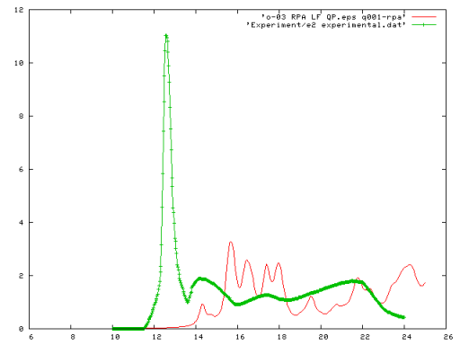
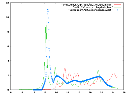
The comparison with the experiment clearly show that the RPA is not at all adequate in the case of LiF. We notice two main discrepancies between theory and experiment: the RPA absorption onset is too low and the shape lacks the sharp peak observed experimentally at around 12 eV. The onset position can be artificially corrected using a scissor operator (representing the QP gap correction) of 5.19 eV that simply opens rigidly the LDA gap. This is shown in Inputs/03_RPA_LF_QP with the line
% XfnQP_E
 5.190000 | 1.000000 | 1.000000 |      # [EXTQP Xd] E parameters (c/v)
%
The resulting spectrum fits better with the experiment but now there seems to be an even more serious problem:
there is an experimental peak well below the QP absorption onset:
an EXCITON!
ALDA (yambo -o c -k alda)
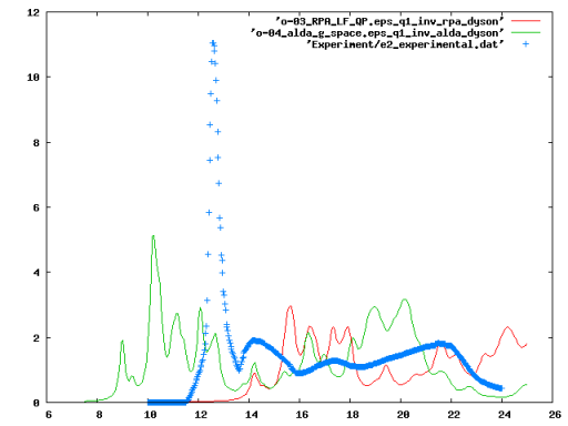
Our first attempt to go beyond RPA is using TDDFT in the Adiabatic LDA approximation. Depending on the exchange-correlation(xc) functional used in the ground state calculation yambo will produce a corresponding xc-kernel. In this case, as reported by the a2y command we are using a Perdew Wang parametrization.
Running
localhost:>yambo -F Inputs/04_alda_g_space -J 04_alda_g_space
we get
Unfortunately ALDA only slightly changes the RPA result. The situation will change in more isolated system (reduced dimensionality).
The Statically screened Electron-electron interaction (yambo -X s)
As simple RPA and ALDA approximations have not described correctly the experimental spectrum we have to move towards more elaborate techniques like the Bethe-Salpeter (BS) equation.
A key ingredient in the BS kernel is the electron-electron interaction commonly evaluated in the static approximation. The input file Inputs/05_W describes how to calculate it. The variables used in this input file have the same physical meaning of those used in the optical absorption calculation. The only difference is that, in general, the response function dimension obtained in the examples (03-04), gives an upper bound to the number of RL vectors needed here. This is because the size of response matrix in an RPA calculation defines also the size of the Hartree potential, whose short-range components are not screened. In the present case, instead, the electron-electron interaction is screened and, for this reason, the RL vectors needed are considerably smaller than in the RPA case. So let's type (no -J option here) ...
localhost:>yambo -F Inputs/05_W
... and after waiting for some minutes the result, that is the database SAVE/ndb.em1s. Do not use the -J option here as we will need to read this database in the next examples.
The Bethe-Salpeter equation, Excitons (yambo -o b -k sex -y h)
The input file Inputs/06_BSE describes how to calculate an excitonic absorption spectrum, by solving the BS equation using the recursive Haydock Method. Before running yambo we must have a closer look at the input file:
The line
% KfnQP_E
 5.80000 | 1.000000 | 1.000000 |      # [EXTQP BSK BSS] E parameters (c/v)
%
applies a 5.8 eV scissor in order to open the LDA gap.
BSKmod= "SEX" # [BSE] IP/Hartree/HF/ALDA/SEX
Here we are using the screened exchange (SEX) approximation for the kernel that includes both exchange and correlation terms
% BSEBands
  2 |  7 |                   # [BSK] Bands range
%
BSENGBlk=  51            RL  # [BSK] Screened interaction block size
BSENGexx=  773           RL  # [BSK] Exchange components
Here we specify the range of bands to be used and the RL components for the screened interaction (51) (read from the ndb.em1s file) and for the Hartree term (773, the maximal available). Remember that the BS kernel is written in Bloch space and its size is given by
BS kernel size = Valence Bands × Conduction Bands × K-points in the whole BZ
In our case the size is 2304. The BS bands range must be converged with care trying to keep as a few bands as possible. Running
localhost:>yambo -F Inputs/06_BSE -J 06_BSE
will calculate the BS kernel and store in in the 06_BSE folder. Before analyzing the BS absorption spectrum we can edit the log file l-06_BSE_optics_bse_bss to observe the on-the-fly live timing feature of yambo:
 [...]
  <---> BSK |                    | [000%] --(E) --(X)
 <05s> BSK |#                   | [007%] 05s(E) 01m-07s(X)
 <11s> BSK |###                 | [015%] 10s(E) 01m-06s(X)
 [...]
 <01m-02s> BSK |##################  | [093%] 01m-01s(E) 01m-06s(X)
 <01m-07s> BSK |####################| [100%] 01m-06s(E) 01m-06s(X)
 [...]
The two numbers at the end of each line represents the elapsed time(E) and the expected time(X). The latter estimates the time needed to complete that particular section (the BS kernel construction in this case).
Finally we can compare the resulting BS optical absorption with the experimental result. We see how strong is the excitonic effect, if compared to the RPA calculation. The BS equation is, then, able to describe the bound electron-hole state responsible for the peak observed experimentally below the QP gap.
A Bethe-Salpeter based Fxc(yambo -o c -k lrc)
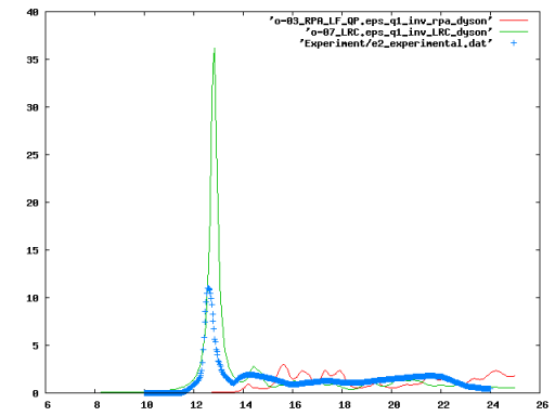
As for TDDFT we might be a little bit disappointed at this stage as the only method that yields a reasonable absorption spectrum for LiF is based on MBPT. It is possible, however, to extract from the BS kernel a possible approximation for the xc-kernel. This approach is efficient, but is far too complicated, and requires the prior computation of the BS kernel. An alternative possibility is to use a simple Long Range Component model, as introduced in Reining. In this model, the yambo input file Inputs/07_LRC describes a model where
We see from the previous figure that the agreement with the BS calculation is not very good. Nevertheless this simple model captures the presence of an exciton and works quite well for a large number of simple semiconductors, as show in Botti:
Additional Exercises
- Calculate the absorption spectra like in section 02-03 increasing the polarization RL size, the polarization bands to find the converged values.
- Plot the EELS spectrum obtained in section 02-03 and check the effect of increasing the polarization bands. Do a resonant only calculation (using the -V option) to see that the EELS cannot be described using only the resonant part of the response function.
See the effect of using a denser BZ sampling grid running Abinit with, for example
ngkpt2 6 6 6
- Repeat the BSE calculation increasing the bands.
- Calculate the BSE spectrum using a diagonal only interaction.
References
- ↑ 1.0 1.1 LiF on wikipedia.
- ↑ 2.0 2.1 M. Rohlfing, S. Louie, Phys. Rev. Lett. 81, 2312 (2000).
- ↑ A. Marini, R. Del Sole, and A. Rubio, Phys. Rev. Lett., 91, 256402 (2003),G. Adragna, R. Del Sole, and A. Marini, Phys. Rev. B 68, 165108 (2003), F. Sottile, V. Olevano, and L. Reining, Phys. Rev. Lett. 91, 056402 (2003).
- ↑ Reining, V. Olevano, A. Rubio, and G. Onida, Phys. Rev. Lett. 88, 066404 (2002).
- ↑ S. Botti, Phys. Rev. B 69, 155112 (2004).
