How to analyse excitons
In this tutorial you will learn (for a 2D-hBN) how to:
- analyze a BSE optical spectrum in terms of excitonic eigenvectors and eigenvalues
- look at the spatial distribution of the exciton
- For a similar tutorial focusing on 3D-hBN, go to this page.
Prerequisites
Previous modules
- You must have completed the How to treat low dimensional systems tutorial
You will need:
yppexecutablexcrysdenexecutablegnuplot or xmgraceexecutable
YAMBO calculations
If you have completed the tutorials of 2D hBN you should have all the databases required to do this tutorial in your YAMBO_TUTORIALS/hBN-2D/SAVE and 2D_WR_WC (databases generated with RIM and cutoff) directories
$ ls ./SAVE
ndb.gops ndb.kindx ns.db1  ns.kb_pp_pwscf_fragment_1 ....
$ ls ./2D_WR_WC
ndb.BS_Q1_CPU_0	ndb.cutoff	ndb.dip_iR_and_P_fragment_1	ndb.pp_fragment_1 ...
Sort the excitonic eigenvalues
$ ypp -J 2D_WR_WC -e s 1
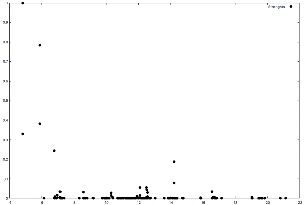
We are sorting the excitons for the q-index = 1 (optical limit q=0). The new generated file o-2D_WR_WC.exc_qpt1_E_sorted (o-2D_WR_WC.exc_qpt1_I_sorted ) reports the energies of the excitons and their Dipole Oscillator Strengths sorted by energy (Index).
Open the first file and look inside. The first exciton is at 4.83 eV and the second one has the highest strength (normalized to 1)
Or you can make a plot
$ gnuplot
gnuplot> set style line 2 lc rgb 'black' pt 7 # circle gnuplot> plot 'o-2D_WR_WC.exc_qpt1_E_sorted' with points ls 2 title 'Strenghts'
Attention the convergence of these results with different k-points grids is mandatory!
Calculate the exciton oscillator strenght and amplitude
We can now analyze the excitons in terms of single-particle states, to do that create the appropriate input
$ ypp -F ypp_AMPL.in -J 2D_WR_WC -e a 1
Suppose you wish to analyze the first 5 excitons then change this line as:
States= "1 - 5" # Index of the BS state(s)
Close the input and run ypp
$ ypp -F ypp_AMPL.in -J 2D_WR_WC
$ls  o*exc*at*
o-2D_WR_WC.exc_qpt1_amplitude_at_1 o-2D_WR_WC.exc_qpt1_weights_at_1 ...
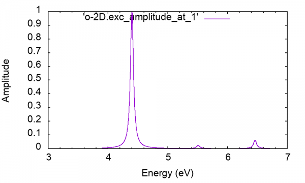
For an exciton [math]\displaystyle{ |\lambda\gt }[/math] , o-2D_WR_WC.exc_qpt1_weights_at_* report the Weights
and o-2D_WR_WC.exc_qpt1_amplitude_** report the amplitudes
Open the file o-2D_WR_WC.exc_weights_at_1
#  Band_V     Band_C     K  ibz     Symm.      Weight     Energy
#
 4.000000   5.000000   7.000000   2.000000   0.922095   4.401093
 4.000000   5.000000   7.000000   1.000000   0.922086   4.401093
The first exciton is  essentially done of only single particle transitions from VBM to CBM at K (last k-point of the grid).
Plot the exciton spatial distribution
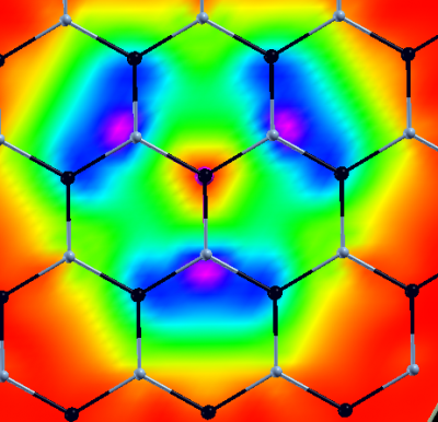
To see the spatial character of the exciton YPP writes the exciton spatial distribution, in other words the probability to find the electron somewhere in the space when the hole is fixed in a give position. Different output formats can be selected and 1D,2D,3D plots done. Create the input and change the size of the cell where to see the exciton. Note that If the k-grid of the BSE simulation is a NxNx1 the exciton has an induced fictitious periodicity every Nx Nx1 Cell of the simulation. For hBN-2D this is not a problem because the exciton is strongly localized but in other systems with more delocalized excitons to look at the real exciton size it is necessary to use very large k-grids in the BSE
$ ypp -F ypp_WF.in -J 2D_WR_WC -e w 1
excitons                     # [R] Excitons
wavefunction                 # [R] Wavefunction
Format= "x"                  # Output format [(c)ube/(g)nuplot/(x)crysden]
Direction= "12"               # [rlu] [1/2/3] for 1d or [12/13/23] for 2d [123] for 3D
FFTGvecs=  3951        RL    # [FFT] Plane-waves
States= "1 - 1"              # Index of the BS state(s)
Degen_Step=   0.0100   eV    # Maximum energy separation of two degenerate states
% Cells
 5 | 5 | 1 |                             # Number of cell repetitions in each direction (odd or 1)
%
% Hole
2.4     | 1.400     | 0.00     |        # [cc] Hole position in unit cell
Close the input and run ypp
$ ypp -F ypp_WF.in -J 2D_WR_WC
$ xcrysden --xsf o-2D_WR_WC.exc_2d_1.xsf
Plot electron/hole average density (only in Yambo 5.x)
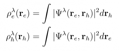
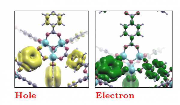
Another way to analyze excitons, it is the possibility to plot the average electron/hole densities defined as:
to generate the corresponding input just type
ypp -F ypp_WF.in -e w -avehole
and choose the exciton you want to plot. The electron/hole average densities correspond to generalized valence/conduction orbitals for a given exciton. They are interesting in particular for molecular crystals because they allow to distinguishing charge-transfer exctions from Frenkel or Wannier ones, by looking the relative position of the electron/hole densities. For example see the electron/hole average density calculated in a Metal Organic Framework (MOF) that contains azobenzene:
this figure is taken from ref. [1].
Interpolate exciton dispersion (only in Yambo 5.x)
Starting from Yambo 5.x it is possible to calculate excitons at finite momentum q. The momentum can be specified with the variable
%BSEQptR
 iq_start | iq_end |                             # [BSK] Transferred momenta range
%
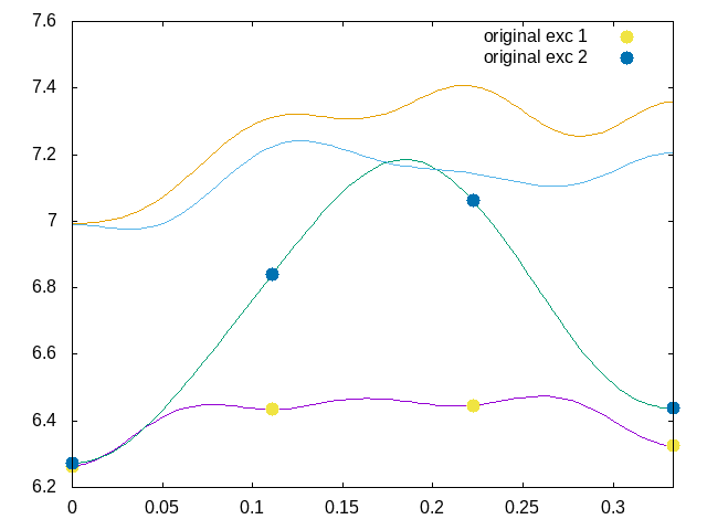
where iq_start and iq_end is the first and last index of momentum in the irreducible Brillouin zone (IBZ). You can find the list of q-vectors in the r_setup report. If you calculate the BSE for all q-points of the IBZ, then you can interpolate exciton dispersion along any direction of the full Brillouin zone(BZ) using the interpolation scheme of ref. [2], by doing:
ypp -e i
and then setting:
excitons                         # [R] Excitonic properties
interpolate                      # [R] Interpolate
States= "1 - 4"                  # Index of the BS state(s)
INTERP_mode= "BOLTZ"                # Interpolation mode (NN=nearest point, BOLTZ=boltztrap aproach)
% INTERP_Grid
 -1 |-1 |-1 |                             # Interpolation BZ Grid
%
#PrtDOS                          # Print Exciton Density of States
BANDS_steps= 100                 # Number of divisions
cooIn= "rlu"                     # Points coordinates (in) cc/rlu/iku/alat
cooOut= "rlu"                    # Points coordinates (out) cc/rlu/iku/alat
%BANDS_kpts                      # K points of the bands circuit
0 | 0 | 0 |
0.333333333333333 | 0.33333333333333 | 0 |
%
Running ypp, it will interpolate the first 4 excitons energies on 100 points along with the line Gamma->K. If you plot the output file "o.excitons_interpolated", you can compare the interpolated results with the original points calculated in the BSE, that are available in the report "r_excitons_interpolate", and you get something like:
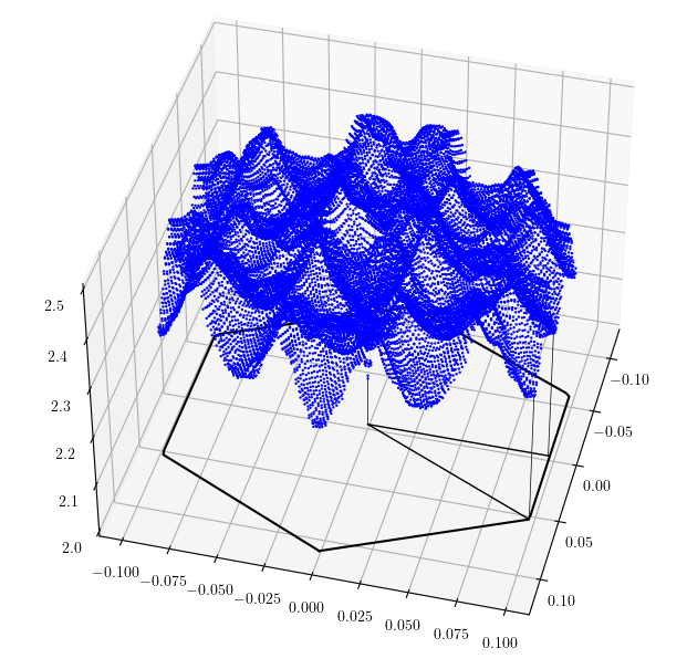
It is also possible to interpolate excitons on a given regular grid by setting INTERP_Grid, for example in the figure below we interpolate the dispersion of the lowest exciton in MoS2 calculated on a 39x39x1 and interpolated in a 117x117x1 grid in all the Brillouin zone:
Finally if you turn on the flag PrtDOS the code calculate the excitonic density of states on the excitons interpolated on the regular grid given by INTERP_Grid.
References
- ↑ Strongly Bound Excitons in Metal-Organic Framework MOF-5: A Many-Body Perturbation Theory Study, A. R. Kshirsagar et al., preprint ChemRxiv
- ↑ Warren E. Pickett, Henry Krakauer, and Philip B. Allen PRB 38 p2721 (1988)

