Real time approach to linear response
Introduction
In this example, we will consider a single layer of hexagonal boron nitride (hBN). If you didn't before you can download input files and Yambo databases for this tutorial here: hBN-2D-RT.tar.gz. and/or follow the instructions to generate the databases here: Prerequisites for Real Time propagation with Yambo
Before proceeding with the real-time simulations it is useful to compute the Independent Particles (IP) absorption spectrum of hBN along the y direction. If you didn't before create an Inputs folder and then the input file with the commands
mkdir Inputs
yambo_nl -o c -F Inputs/01_ip.in
and set the proper input parameters
 optics                         # [R OPT] Optics
 chi                            # [R CHI] Dyson equation for Chi.
 dipoles                        # [R   ] Compute the dipoles
 Chimod= "IP"                   # [X] IP/Hartree/ALDA/LRC/PF/BSfxc
 % QpntsRXd
    1 |  1 |                   # [Xd] Transferred momenta
 %
 % BndsRnXd
   3 | 6 |                     # [Xd] Polarization function bands
 %
 % EnRngeXd
   0.00000 | 20.00000 | eV      # [Xd] Energy range
 %
 % DmRngeXd
   0.10000 |  0.10000 | eV      # [Xd] Damping range
 %
 ETStpsXd= 2001                  # [Xd] Total Energy steps
 % LongDrXd
  0.000000 | 1.000000 | 0.000000 |        # [Xd] [cc] Electric Field
 %
and then run the code
yambo_nl -F Inputs/01_ip.in -J CHI_IP -C CHI_IP
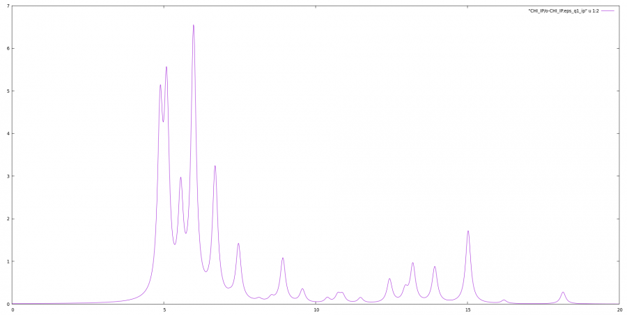
The resulting spectrum will give an idea of the energy involved in the real-time simulations
gnuplot
gnuplot> plot "CHI_IP/o-CHI_IP.eps_q1_ip" u 1:2 w l
Real-time dynamics at the independent particles level
Since we work with the two independent approaches coded in yambo it will be useful to create two different folders for the input files.
mkdir Inputs_rt
mkdir Inputs_nl
In order to calculate linear-response in real-time, we will perturb the system with a delta function in time external field.
Approach based on the density matrix
Use the command
yambo_rt -n p -F Inputs_rt/01_td_ip.in
to generate the input:
 negf                           # [R] Real-Time dynamics
 RT_Threads=0                   # [OPENMP/RT] Number of threads for real-time
 HXC_Potential= "IP"           # [SC] SC HXC Potential
 % RTBands
   3 |  6 |                     # [RT] Bands
 %
 Integrator= "EULER RK2"              # [RT] Integrator. Use keywords space separated  ( "EULER/EXPn/INV" "SIMPLE/RK2/RK4/HEUN" "RWA")
 PhLifeTime= 0.000000   fs      # [RT] Dephasing Time
 RTstep=10.000000       as      # [RT] Real Time step length
 NETime= 55.00000       fs      # [RT] Simulation Time
 % IOtime
  0.05     | 5.00     | 0.10     |  fs    # [RT] Time between to consecutive I/O (OBSERVABLEs,CARRIERs - GF - OUTPUT)
 %
 % Field1_Freq
  0.00     | 0.00     | eV      # [RT Field1] Frequency
 %
 Field1_Int=1.E3   kWLm2   # [RT Field1] Intensity
 Field1_Width= 0.000000 fs      # [RT Field1] Width
 Field1_kind= "DELTA"           # [RT Field1] Kind(SIN|RES|ANTIRES|GAUSS|DELTA|QSSIN)
 Field1_pol= "linear"           # [RT Field1] Pol(linear|circular)
 % Field1_Dir
  0.000000 | 1.000000 | 0.000000 |        # [RT Field1] Versor
 %
 % Field1_Dir_circ
  0.000000 | 1.000000 | 0.000000 |        # [RT Field1] Versor_circ
 %
 Field1_Tstart= 0.000000fs      # [RT Field1] Initial Time
Set the field direction along y, the field type to DELTA, the length of the simulation to 55 fs, number of bands from 3 to 6, dephasing to zero and the field intensity to 1.E3 [kW/cm2].
A small intensity is needed to ensure that we remain in the perturbative regime and that the response is dominated by linear term.
The yambo_rt is optimized for TD-SEX (or even more sophisticated calculations).
Now run the simulation:
yambo_rt -F Inputs_rt/01_td_ip.in -J TD-IP_rt -C TD-IP_rt
The run produces, besides the standard report and (eventually) log files of yambo, 3 output files:
 TD-IP_rt/01_td_ip.in_TD-IP_rt
 TD-IP_rt/r-TD-IP_rt_negf
 TD-IP_rt/o-TD-IP_rt.polarization
 TD-IP_rt/o-TD-IP_rt.external_field
 TD-IP_rt/o-TD-IP_rt.current
Moreover it also makes a copy of the input file. If the run is taking to long you can open the copy of the input file TD-IP_rt/01_td_ip.in_TD-IP_rt and add there the string
STOP_NOW
It will finish the simulation in a proper way.
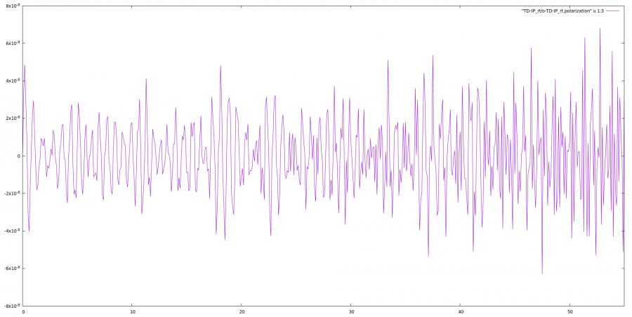
You can now plot the resulting time-dependent polarization and obtain something like this
gnuplot
plot "TD-IP_rt/o-TD-IP_rt.polarization" u 1:3 w l
The polarization is oscillating very quickly and with the time step for the output file we have chosen (100 as) we can hardly resolve the oscillations. The slowest oscillation is expected at the first absorption peak, which is located slightly above 4 eV. This corresponds to a period of about 1 fs. Higher energy transitions are however also activated by the delta like pulse, which spans all frequencies (remember that the Fourier transform of a delta function is a constant).
The I/O time, which is negligible in such calculations, is less optimized and becomes the most time demanding step here. We can overcome this setting the IOtime for the polarization to 50 as (i.e. each 5 time steps). After the run you can have a look at the timing report and you will see that indeed most of the timing was spent in the I/O:
RT databases IO : 6.8745 s CPU ( 5501 calls, 0.0012 s avg)
Approach based on the Berry Phase
Use the command
yambo_nl -u -F Inputs_nl/01_td_ip.in
to generate the input:
nloptics                      # [R NL] Non-linear optics
NL_Threads= 1                # [OPENMP/NL] Number of threads for nl-optics
% NLBands
  3 |  6 |                   # [NL] Bands
%
NLstep=   0.0100       fs    # [NL] Real Time step length
NLtime=55.000000      fs    # [NL] Simulation Time
NLverbosity= "high"           # [NL] Verbosity level (low | high)
NLintegrator= "INVINT"       # [NL] Integrator ("EULEREXP/RK4/RK2EXP/HEUN/INVINT/CRANKNIC")
NLCorrelation= "IPA"         # [NL] Correlation ("IPA/HARTREE/TDDFT/LRC/JGM/SEX/HF")
NLLrcAlpha= 0.000000         # [NL] Long Range Correction
% NLEnRange
 0.200000 | 8.000000 | eV    # [NL] Energy range
%
NLEnSteps= 1                 # [NL] Energy steps
NLDamping= 0.000000    eV    # [NL] Damping
% ExtF_Dir
 0.000000 | 1.000000  | 0.000000 |        # [NL ExtF] Versor
%
ExtF_kind=  "DELTA"          # [NL ExtF] Kind(SIN|SOFTSIN|RES|ANTIRES|GAUSS|DELTA|QSSIN)
The standard input of yambo_nl is thought for the non-linear response so we have to change some parameters in order to calculate the linear response. Set the field direction along y, the field type to DELTA, the length of the simulation to 55 fs, number of bands from 3 to 6 dephasing to zero and the number of energy steps to one, as shown above in red.
We set the verbosity to "high" in such a way to print real-time output files.
We set the differential equation integrator to INVINT that is faster but less accurate than the default (see Ref. [1]) . This integrator is ok in case of independent particles but I advise you to use CRANKNIC integrator when correlation effects are present.
Now run
yambo_nl -F Inputs_nl/01_td_ip.in -J TD-IP_nl -C TD-IP_nl
The code will produce different files: o.polarization_F1 that contains the polarization, o.external_potential_F1 the external field we used, and finally r_optics_nloptics a report with all information about the simulation.
This time the simulation took much longer. This is the price to pay for computing the polarization with the Berry Phase technique. While there is no much gain in linear response, this will allow to compute also non linear coefficients which cannot be obtained with the density based approach. If we look at the time profile of the run we see:
 NL Berry Pol NEQ :  313.5414 s CPU (    5502 calls,    0.0570 s avg)
 SERIAL_inversion :  307.3369 s CPU ( 4402840 calls,    0.0001 s avg)
    NL Integrator :   87.6024 s CPU (    5501 calls,    0.0159 s avg)
SERIAL_lin_system :   85.9291 s CPU ( 1210220 calls,    0.0001 s avg)
Most of the time is spent computing the non-equilibrium Berry Polarization, which involves the inversion of small matrices via the Lapack inversion routine. Some time is also required by the inversion solved which is coded via the solution of a linear system of equations as implemented in the Lapack library. This integrator is more accurate than the Runge-Kutta 2nd order employed previously
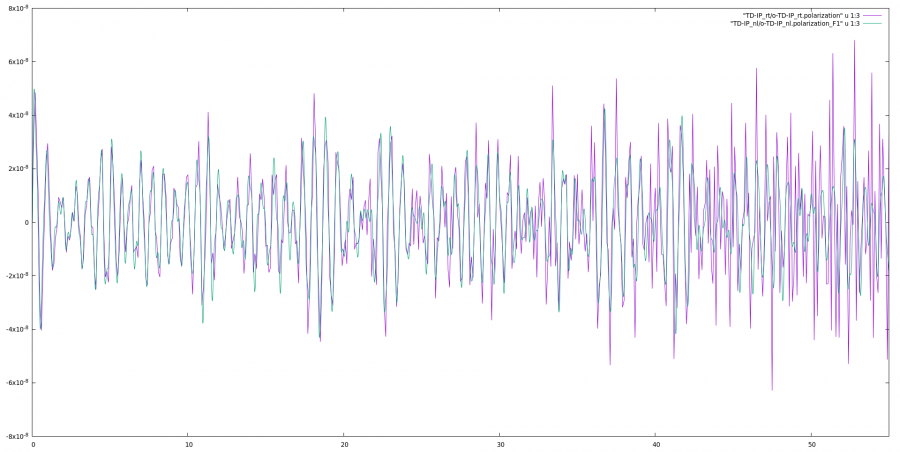
If you plot the third column of o.polarization_F1 versus the first one (time-variable) you will get the time-dependent polarization along the y-direction:
In the plot the polarization from the two different propagation schemes are compared. There are few differences which could be due to the following reasons:
- Coupling with the external field: the
yambo_rtevaluates the coupling with the external field through the dipoles (by default computing the commutator [x,Hnl]; theyambo_nlevaluates the coupling using an expression based on the Berry Phase. For the latter, a numerical differentiation in reciprocal space is performed. The 10x10 2D k-mesh may not be fine enough. For denser k-mesh, the Berry phase approach converges to the one based on the dipoles. To avoid this one can useDipApproach="Covariant"in the scheme used by yambo_rt. - Integrator: the integrator used for the
yambo_nlis more accurate. The fact that the differences are more pronounced for long times may hint to inaccuracies in the integration of the equation of motions inyambo_rt. One can use a similar integrator with yambo_rt, by setting in inputIntegrator= "INV RK2"
Results Analysis
We can now proceed to the Fourier transform of the polarization to obtain the dielectric function
Approach based on the density matrix
Now we can use
ypp_rt -t X -F Inputs_rt/ypp_abs.in
to generate the input file
 RealTime                       # [R] Real-Time Post-Processing
 RT_X                           # [R] Response functions Post-Processing
 Xorder=1                       # Max order of the response/exc functions
 % EnRngeRt
  0.00     | 10.00     | eV      # Energy range
 %
 ETStpsRt=1001                     # Total Energy steps
 % TimeRange
  0.00     | 0.00     | fs      # Time-window where processing is done
 %
DampMode= "LORENTZIAN"             # Damping type ( NONE | LORENTZIAN | GAUSSIAN )
DampFactor=  0.10000   eV    # Damping parameter
where we set a Lorentzian smearing corresponding to 0.1 eV. Notice that due to the finite time of our simulation smearing is always necessary to Fourier transform the result. Then we run
ypp_rt -F Inputs_rt/ypp_abs.in -J TD-IP_rt -C TD-IP_rt
and obtain the files for the dielectric constant along with the field direction, the EELS along with the same direction, and the damped polarization.
o-TD-IP_rt.YPP-eps_along_E
o-TD-IP_rt.YPP-eels_along_E
o-TD-IP_rt.YPP-polarization
o-TD-IP_rt.YPP-current
o-TD-IP_rt.YPP-E_frequency
inside the folder TD-IP_rt
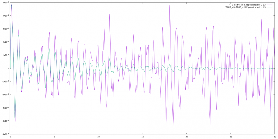
First let's have a look to the polarization.
gnuplot
plot "TD-IP_rt/o-TD-IP_rt.polarization" u 1:3 w l
replot "TD-IP_rt/o-TD-IP_rt.YPP-polarization" u 1:3 w l
We clearly see the effect of the Lorentzian damping added to the time dependent polarization
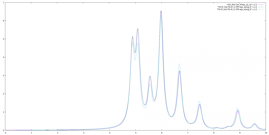
Now we can plot the dielectric constant and compare it with the linear response:
Approach based on the Berry Phase
Now we can use
ypp_nl -u -F Inputs_nl/ypp_abs.in
to generate the input file:
nonlinear                    # [R] NonLinear Optics Post-Processing
Xorder= 1                    # Max order of the response functions
% TimeRange
-1.000000 |-1.000000 | fs    # Time-window where processing is done
%
ETStpsRt= 1001                # Total Energy steps
% EnRngeRt
  0.00000 | 10.00000 | eV    # Energy range
%
DampMode= "LORENTZIAN"             # Damping type ( NONE | LORENTZIAN | GAUSSIAN )
DampFactor=  0.10000   eV    # Damping parameter
where we set a Lorentzian smearing corresponding to 0.1 eV. Notice that due to the finite time of our simulation smearing is always necessary to Fourier transform the result.
Then we run
ypp_nl -F Inputs_nl/ypp_abs.in -J TD-IP_nl -C TD-IP_nl
and obtain the files for the dielectric constant along with the field direction, the EELS along with the same direction, and the damped polarization.
o-TD-IP_nl.YPP-eps_along_E
o-TD-IP_nl.YPP-eels_along_E
o-TD-IP_nl.YPP-damped_polarization
inside the folder TD-IP_nl
Now we can plot the dielectric constant and compare it with the linear response:
gnuplot
plot "CHI_IP/o-CHI_IP.eps_q1_ip" u 1:2 w l
rep "TD-IP_rt/o-TD-IP_rt.YPP-eps_along_E" u 1:2 w l
rep "TD-IP_nl/o-TD-IP_nl.YPP-eps_along_E" u 1:2 w l
At low energy the post processing of yambo_rt are closer to the linear response approach, since they both share the same dipoles. At higher energies however the post processing of yambo_nl gives a better description of the energies, probably due to the better integrator. One can try to use the inversion integrator with yambo_rt or the covariant dipoles in linear response to better understand these differences.
More info on this tutorial can be found in here.
| Prev: Prerequisites | Now: Tutorials --> Linear Response --> Independent Particles | Next: Real time Bethe-Salpeter Equation (TDSE) |
- ↑ C. Attaccalite and M. Gruning Rev. B, 88, 235113 (2013)
